13 Case Study in Data Wrangling
13.1 Yeast Genomics
Smith and Kruglyak (2008) is a study that measured 2820 genotypes in 109 yeast F1 segregants from a cross between parental lines BY and RM.
They also measured gene expression on 4482 genes in each of these segregants when growing in two different Carbon sources, glucose and ethanol.
13.1.1 Load Data
The data was distributed as a collection of matrices in R.
> rm(list=ls())
> load("./data/smith_kruglyak.RData")
> ls()
[1] "exp.e"      "exp.g"      "exp.pos"    "marker"     "marker.pos"
> eapply(env=.GlobalEnv, dim)
$exp.e
[1] 4482  109

$exp.g
[1] 4482  109

$marker
[1] 2820  109

$exp.pos
[1] 4482    3

$marker.pos
[1] 2820    2
13.1.2 Gene Expression Matrices
> exp.g %>% cbind(rownames(exp.g), .) %>% as_tibble() %>%
+   print()
Warning: `as_tibble.matrix()` requires a matrix with column names or a `.name_repair` argument. Using compatibility `.name_repair`.
This warning is displayed once per session.
# A tibble: 4,482 x 110
   V1    X100g.20_4_c.gl… X101g.21_1_d.gl… X102g.21_2_d.gl…
   <chr> <chr>            <chr>            <chr>
 1 YJR1… 0.22             0.18             0.05
 2 YPL2… -0.29            -0.2             -0.19
 3 YDR5… 0.72             0.04             0.26
 4 YDR2… 0.23             0.31             0.12
 5 YHR0… 0.4              -0.04            0.36
 6 YFR0… -0.36            0.35             -0.26
 7 YPL1… 0.23             -0.21            -0.25
 8 YDR0… -0.09            0.57             0.24
 9 YLR3… -0.23            0.13             -0.17
10 YCR0… -0.25            -0.98            -0.3
# … with 4,472 more rows, and 106 more variables:
#   X103g.21_3_d.glucose <chr>, X104g.21_4_d.glucose <chr>,
#   X105g.21_5_c.glucose <chr>, X106g.22_2_d.glucose <chr>,
#   X107g.22_3_b.glucose <chr>, X109g.22_5_d.glucose <chr>,
#   X10g.2_5_d.glucose <chr>, X110g.23_3_d.glucose <chr>,
#   X111g.23_5_d.glucose <chr>, X112g.24_1_d.glucose <chr>,
#   X113g.25_1_d.glucose <chr>, X114g.25_3_d.glucose <chr>,
#   X115g.25_4_d.glucose <chr>, X116g.26_1_d.glucose <chr>,
#   X117g.26_2_d.glucose <chr>, X11g.2_6_d.glucose <chr>,
#   X12g.2_7_a.glucose <chr>, X13g.3_1_d.glucose <chr>,
#   X15g.3_3_d.glucose <chr>, X16g.3_4_d.glucose <chr>,
#   X17g.3_5_d.glucose <chr>, X18g.4_1_c.glucose <chr>,
#   X1g.1_1_d.glucose <chr>, X20g.4_3_d.glucose <chr>,
#   X21g.4_4_d.glucose <chr>, X22g.5_1_d.glucose <chr>,
#   X23g.5_2_d.glucose <chr>, X24g.5_3_d.glucose <chr>,
#   X25g.5_4_d.glucose <chr>, X26g.5_5_d.glucose <chr>,
#   X27g.6_1_d.glucose <chr>, X28g.6_2_b.glucose <chr>,
#   X29g.6_3_c.glucose <chr>, X30g.6_4_d.glucose <chr>,
#   X31g.6_5_d.glucose <chr>, X32g.6_6_d.glucose <chr>,
#   X33g.6_7_d.glucose <chr>, X34g.7_1_d.glucose <chr>,
#   X35g.7_2_c.glucose <chr>, X36g.7_3_d.glucose <chr>,
#   X37g.7_4_c.glucose <chr>, X38g.7_5_d.glucose <chr>,
#   X39g.7_6_c.glucose <chr>, X3g.1_3_d.glucose <chr>,
#   X40g.7_7_c.glucose <chr>, X41g.7_8_d.glucose <chr>,
#   X42g.8_1_a.glucose <chr>, X43g.8_2_d.glucose <chr>,
#   X44g.8_3_a.glucose <chr>, X45g.8_4_c.glucose <chr>,
#   X46g.8_5_b.glucose <chr>, X47g.8_6_c.glucose <chr>,
#   X48g.8_7_b.glucose <chr>, X49g.9_1_d.glucose <chr>,
#   X4g.1_4_d.glucose <chr>, X50g.9_2_d.glucose <chr>,
#   X51g.9_3_d.glucose <chr>, X52g.9_4_d.glucose <chr>,
#   X53g.9_5_d.glucose <chr>, X54g.9_6_d.glucose <chr>,
#   X55g.9_7_d.glucose <chr>, X56g.10_1_c.glucose <chr>,
#   X57g.10_2_d.glucose <chr>, X58g.10_3_c.glucose <chr>,
#   X59g.10_4_d.glucose <chr>, X5g.1_5_c.glucose <chr>,
#   X60g.11_1_a.glucose <chr>, X61g.11_2_d.glucose <chr>,
#   X62g.11_3_b.glucose <chr>, X63g.12_1_d.glucose <chr>,
#   X64g.12_2_b.glucose <chr>, X65g.13_1_a.glucose <chr>,
#   X66g.13_2_c.glucose <chr>, X67g.13_3_b.glucose <chr>,
#   X68g.13_4_a.glucose <chr>, X69g.13_5_c.glucose <chr>,
#   X70g.14_1_b.glucose <chr>, X71g.14_2_c.glucose <chr>,
#   X73g.14_4_a.glucose <chr>, X74g.14_5_b.glucose <chr>,
#   X75g.14_6_d.glucose <chr>, X76g.14_7_c.glucose <chr>,
#   X77g.15_2_d.glucose <chr>, X78g.15_3_b.glucose <chr>,
#   X79g.15_4_d.glucose <chr>, X7g.2_2_d.glucose <chr>,
#   X80g.15_5_b.glucose <chr>, X82g.16_1_d.glucose <chr>,
#   X83g.17_1_a.glucose <chr>, X84g.17_2_d.glucose <chr>,
#   X85g.17_4_a.glucose <chr>, X86g.17_5_b.glucose <chr>,
#   X87g.18_1_d.glucose <chr>, X88g.18_2_d.glucose <chr>,
#   X89g.18_3_d.glucose <chr>, X8g.2_3_d.glucose <chr>,
#   X90g.18_4_c.glucose <chr>, X92g.19_1_c.glucose <chr>,
#   X93g.19_2_c.glucose <chr>, X94g.19_3_c.glucose <chr>, …
13.1.3 Gene Position Matrix
> exp.pos %>% cbind(rownames(exp.pos), .) %>% as_tibble() %>%
+   print()
# A tibble: 4,482 x 4
   V1      Chromsome Start_coord End_coord
   <chr>   <chr>     <chr>       <chr>
 1 YJR107W 10        627333      628319
 2 YPL270W 16        30482       32803
 3 YDR518W 4         1478600     1480153
 4 YDR233C 4         930353      929466
 5 YHR098C 8         301937      299148
 6 YFR029W 6         210925      212961
 7 YPL198W 16        173151      174701
 8 YDR001C 4         452472      450217
 9 YLR394W 12        907950      909398
10 YCR079W 3         252842      254170
# … with 4,472 more rows
13.1.4 Row Names
The gene names are contained in the row names.
> head(rownames(exp.g))
[1] "YJR107W" "YPL270W" "YDR518W" "YDR233C" "YHR098C" "YFR029W"
> head(rownames(exp.e))
[1] "YJR107W" "YPL270W" "YDR518W" "YDR233C" "YHR098C" "YFR029W"
> head(rownames(exp.pos))
[1] "YJR107W" "YPL270W" "YDR518W" "YDR233C" "YHR098C" "YFR029W"
> all.equal(rownames(exp.g), rownames(exp.e))
[1] TRUE
> all.equal(rownames(exp.g), rownames(exp.pos))
[1] TRUE
13.1.5 Unify Column Names
The segregants are column names, and they are inconsistent across matrices.
> head(colnames(exp.g))
[1] "X100g.20_4_c.glucose" "X101g.21_1_d.glucose" "X102g.21_2_d.glucose"
[4] "X103g.21_3_d.glucose" "X104g.21_4_d.glucose" "X105g.21_5_c.glucose"
> head(colnames(marker))
[1] "20_4_c" "21_1_d" "21_2_d" "21_3_d" "21_4_d" "21_5_c"
>
> ##fix column names with gsub
> colnames(exp.g) %<>% strsplit(split=".", fixed=TRUE) %>%
+   lapply(function(x) {x[2]})
> colnames(exp.e) %<>% strsplit(split=".", fixed=TRUE) %>%
+   lapply(function(x) {x[2]})
> head(colnames(exp.g))
[1] "20_4_c" "21_1_d" "21_2_d" "21_3_d" "21_4_d" "21_5_c"
13.1.6 Gene Positions
Let’s first pull out rownames of exp.pos and make them a column in the data frame.
> gene_pos <- exp.pos %>% as_tibble() %>%
+   mutate(gene = rownames(exp.pos)) %>%
+   dplyr::select(gene, chr = Chromsome, start = Start_coord,
+                 end = End_coord)
> print(gene_pos, n=7)
# A tibble: 4,482 x 4
  gene      chr   start     end
  <chr>   <int>   <int>   <int>
1 YJR107W    10  627333  628319
2 YPL270W    16   30482   32803
3 YDR518W     4 1478600 1480153
4 YDR233C     4  930353  929466
5 YHR098C     8  301937  299148
6 YFR029W     6  210925  212961
7 YPL198W    16  173151  174701
# … with 4,475 more rows
13.1.7 Tidy Each Expression Matrix
We melt the expression matrices and bind them together into one big tidy data frame.
> exp_g <- melt(exp.g) %>% as_tibble() %>%
+   dplyr::select(gene = Var1, segregant = Var2,
+                 expression = value) %>%
+   mutate(condition = "glucose")
> exp_e <- melt(exp.e) %>% as_tibble() %>%
+   dplyr::select(gene = Var1, segregant = Var2,
+                 expression = value) %>%
+   mutate(condition = "ethanol")
> print(exp_e, n=4)
# A tibble: 488,538 x 4
  gene    segregant expression condition
  <fct>   <fct>          <dbl> <chr>
1 YJR107W 20_4_c          0.06 ethanol
2 YPL270W 20_4_c         -0.13 ethanol
3 YDR518W 20_4_c         -0.94 ethanol
4 YDR233C 20_4_c          0.04 ethanol
# … with 4.885e+05 more rows
13.1.8 Combine Into Single Data Frame
Combine gene expression data from two conditions into a single data frame.
> exp_all <- bind_rows(exp_g, exp_e)
> sample_n(exp_all, size=10)
# A tibble: 10 x 4
   gene    segregant expression condition
   <fct>   <fct>          <dbl> <chr>
 1 YBL087C 21_4_d         -0.72 ethanol
 2 YDR524C 21_2_d         -0.17 glucose
 3 YGR067C 9_1_d          -3.92 glucose
 4 YHR207C 26_1_d         -0.43 ethanol
 5 YDR329C 20_2_d         -0.06 glucose
 6 YGL121C 8_7_b           1    ethanol
 7 YJR044C 3_3_d          -0.12 ethanol
 8 YIL088C 2_7_a           0.1  ethanol
 9 YML127W 5_1_d          -0.08 ethanol
10 YMR304W 6_1_d           0.2  ethanol
13.1.9 Join Gene Positions
Now we want to join the gene positions with the expression data.
> exp_all <- exp_all %>%
+   mutate(gene = as.character(gene),
+          segregant = as.character(segregant))
> sk_tidy <- exp_all %>%
+   left_join(gene_pos, by = "gene")
> sample_n(sk_tidy, size=7)
# A tibble: 7 x 7
  gene    segregant expression condition   chr  start    end
  <chr>   <chr>          <dbl> <chr>     <int>  <int>  <int>
1 YGL189C 1_3_d          -0.26 ethanol       7 148594 148235
2 YBR257W 13_2_c          0.02 ethanol       2 728880 729719
3 YER098W 21_1_d          0.46 ethanol       5 355462 357726
4 YCR035C 9_1_d           0.07 glucose       3 193014 191830
5 YBR097W 17_5_b         -0.03 glucose       2 436945 441309
6 YBR235W 8_4_c          -0.18 ethanol       2 686896 690258
7 YJL094C 14_6_d          0    glucose      10 254437 251816
13.1.10 Apply dplyr Functions
Now that we have the data made tidy in the data frame sk_tidy, let’s apply some dplyr operations…
Does each gene have the same number of observations?
> sk_tidy %>% group_by(gene) %>%
+   summarize(value = n()) %>%
+   summary()
     gene               value
 Length:4478        Min.   :218.0
 Class :character   1st Qu.:218.0
 Mode  :character   Median :218.0
                    Mean   :218.6
                    3rd Qu.:218.0
                    Max.   :872.0
No, so let’s see which genes have more than one set of observations.
> sk_tidy %>% group_by(gene) %>%
+   summarize(value = n()) %>%
+   filter(value > median(value))
# A tibble: 4 x 2
  gene      value
  <chr>     <int>
1 YFR024C-A   872
2 YJL012C     872
3 YKL198C     872
4 YPR089W     872
Let’s remove replicated measurements for these genes.
> sk_tidy %<>% distinct(gene, segregant, condition,
+                       .keep_all = TRUE)
>
> sk_tidy %>% group_by(gene) %>%
+   summarize(value = n()) %>%
+   summary()
     gene               value
 Length:4478        Min.   :218
 Class :character   1st Qu.:218
 Mode  :character   Median :218
                    Mean   :218
                    3rd Qu.:218
                    Max.   :218
As an exercise, think about how you would use dplyr to replace the replicated gene expression values with a single averaged expression value for these genes.
Get the mean and standard deviation expression per chromosome.
> sk_tidy %>%
+   group_by(chr) %>%
+   summarize(mean = mean(expression), sd=sd(expression))
# A tibble: 16 x 3
     chr    mean    sd
   <int>   <dbl> <dbl>
 1     1 -0.0762 0.826
 2     2 -0.0447 0.632
 3     3 -0.0230 0.682
 4     4 -0.0233 0.537
 5     5 -0.0579 0.610
 6     6 -0.0772 0.660
 7     7 -0.0441 0.617
 8     8 -0.0474 0.638
 9     9 -0.0430 0.614
10    10 -0.0299 0.570
11    11 -0.0396 0.613
12    12 -0.0515 0.643
13    13 -0.0265 0.584
14    14 -0.0294 0.642
15    15 -0.0130 0.554
16    16 -0.0368 0.604
Get the mean and standard deviation expression per chromosome in each condition.
> sk_tidy %>%
+   group_by(chr, condition) %>%
+   summarize(mean = mean(expression), sd=sd(expression))
# A tibble: 32 x 4
# Groups:   chr [?]
     chr condition      mean    sd
   <int> <chr>         <dbl> <dbl>
 1     1 ethanol    0.0260   0.480
 2     1 glucose   -0.178    1.05
 3     2 ethanol    0.0132   0.479
 4     2 glucose   -0.103    0.750
 5     3 ethanol    0.000164 0.536
 6     3 glucose   -0.0461   0.800
 7     4 ethanol    0.00187  0.482
 8     4 glucose   -0.0484   0.586
 9     5 ethanol   -0.0297   0.479
10     5 glucose   -0.0862   0.716
# … with 22 more rows
Count the number of genes per chromosome.
> sk_tidy %>%
+   filter(condition == "glucose", segregant == "20_4_c") %>%
+   group_by(chr) %>%
+   summarize(num.genes = n())
# A tibble: 16 x 2
     chr num.genes
   <int>     <int>
 1     1        60
 2     2       298
 3     3       125
 4     4       629
 5     5       207
 6     6        79
 7     7       395
 8     8       209
 9     9       152
10    10       256
11    11       241
12    12       387
13    13       367
14    14       319
15    15       388
16    16       366
Filter for the first gene on every chromosome.
> sk_tidy %>%
+ filter(condition == "glucose", segregant == "20_4_c") %>%
+ group_by(chr) %>%
+ filter(start == min(start))
# A tibble: 16 x 7
# Groups: chr [16]
gene segregant expression condition chr start end
<chr> <chr> <dbl> <chr> <int> <int> <int>
1 YHL040C 20_4_c -2.79 glucose 8 20968 19085
2 YNL334C 20_4_c -0.9 glucose 14 12876 12208
3 YOL157C 20_4_c -1.06 glucose 15 24293 22524
4 YKL222C 20_4_c 0.09 glucose 11 5621 3504
5 YIL168W 20_4_c -1.14 glucose 9 29032 29415
6 YJL213W 20_4_c 0.84 glucose 10 32163 33158
7 YPL272C 20_4_c -0.18 glucose 16 28164 26611
8 YLL063C 20_4_c -0.66 glucose 12 16072 14648
9 YFL048C 20_4_c -0.09 glucose 6 40180 38843
10 YML132W 20_4_c -0.21 glucose 13 7244 8383
11 YGL261C 20_4_c -0.14 glucose 7 6652 6290
12 YBL107C 20_4_c 0.290 glucose 2 10551 9961
13 YDL248W 20_4_c -0.68 glucose 4 1802 2953
14 YEL073C 20_4_c -0.02 glucose 5 7553 7230
15 YAL062W 20_4_c -5.64 glucose 1 31568 32941
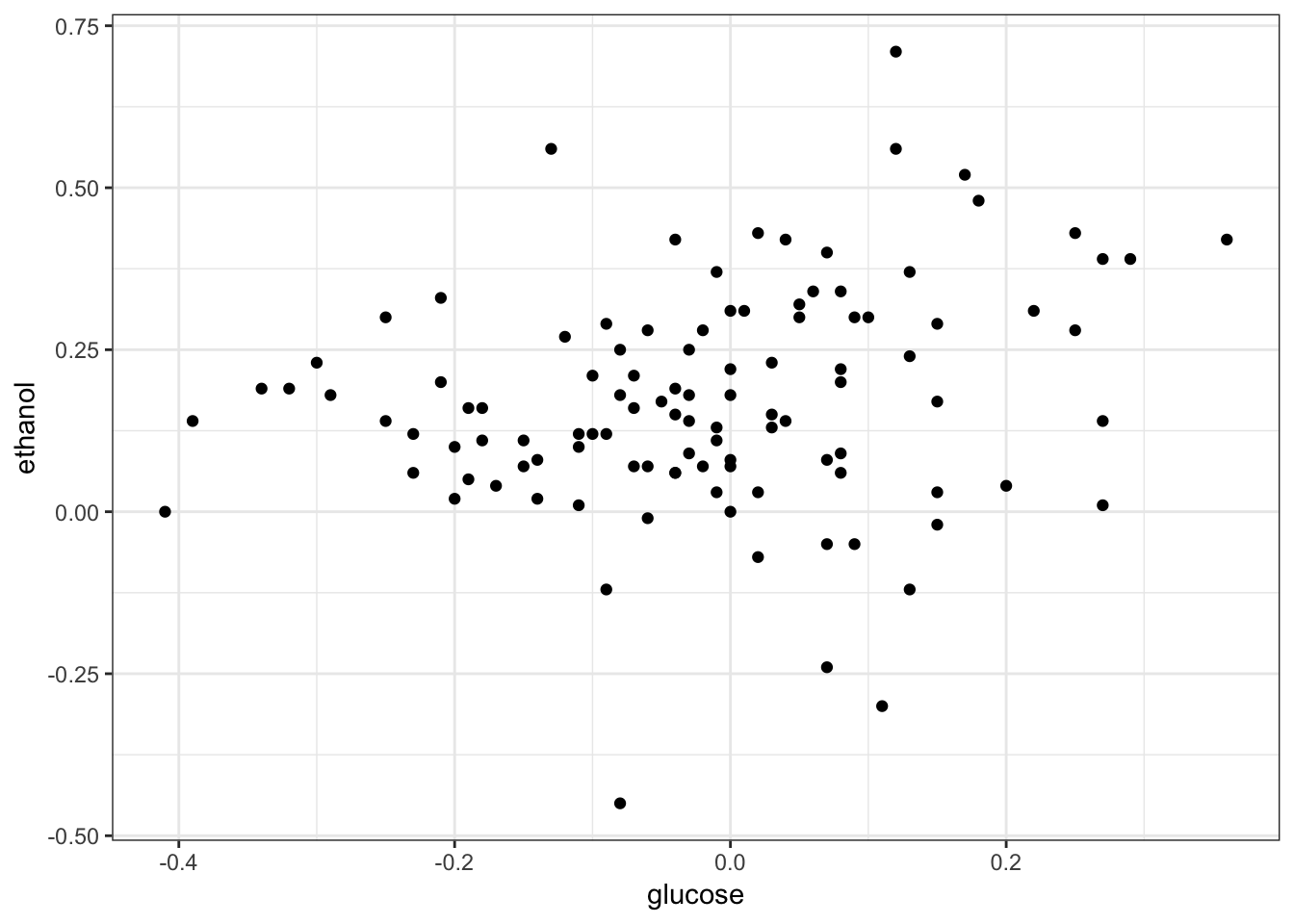
16 YCL068C 20_4_c 0.47 glucose 3 12285 11503To plot expression in glucose versus ethanol we first need to use dcast().
> sk_tidy %>% dcast(gene + segregant ~ condition,
+                   value.var = "expression") %>%
+   as_tibble()
# A tibble: 488,102 x 4
   gene    segregant ethanol glucose
   <chr>   <chr>       <dbl>   <dbl>
 1 YAL002W 1_1_d        0.37   -0.01
 2 YAL002W 1_3_d        0.23    0.03
 3 YAL002W 1_4_d        0.08    0.07
 4 YAL002W 1_5_c       -0.12    0.13
 5 YAL002W 10_1_c       0.12   -0.1
 6 YAL002W 10_2_d       0.1    -0.2
 7 YAL002W 10_3_c       0.07   -0.15
 8 YAL002W 10_4_d       0.06   -0.04
 9 YAL002W 11_1_a       0.07   -0.07
10 YAL002W 11_2_d       0.3     0.1
# … with 488,092 more rows
> sk_tidy %>% dcast(gene + segregant ~ condition,
+ value.var = "expression") %>%
+ filter(gene == "YAL002W") %>%
+ ggplot(aes(x = glucose, y = ethanol)) +
+ geom_point() + theme_bw() +
+ theme(legend.position = "none")