51 Permutation Methods
51.1 Rationale
Permutation methods are useful for testing hypotheses about equality of distributions.
Observations can be permuted among populations to simulate the case where the distributions are equivalent.
Many permutation methods only depend on the ranks of the data, so they are a class of robust methods for performing hypothesis tests. However, the types of hypotheses that can be tested are limited.
51.2 Permutation Test
Suppose \(X_1, X_2, \ldots, X_m {\; \stackrel{\text{iid}}{\sim}\;}F_X\) and \(Y_1, Y_2, \ldots, Y_n {\; \stackrel{\text{iid}}{\sim}\;}F_Y\).
We wish to test \(H_0: F_X = F_Y\) vs \(H_1: F_X \not= F_Y\).
Consider a general test statistic \(S = S(X_1, X_2, \ldots, X_m, Y_1, Y_2, \ldots, Y_n)\) so that the larger \(S\) is the more evidence there is against the null hypothesis.
Under the null hypothesis, any reordering of these values, where \(m\) are randomly assigned to the “\(X\)” population and \(n\) are assigned to the “\(Y\)” population, should be equivalently distributed.
For \(B\) permutations (possibly all unique permutations), we calculate
\[ S^{*(b)} = S\left(Z^{*(b)}_1, Z^{*(b)}_2, \ldots, Z^{*(b)}_m, Z^{*(b)}_{m+1}, \ldots, Z^{*(b)}_{m+n}\right) \]
where \(Z^{*(b)}_1, Z^{*(b)}_2, \ldots, Z^{*(b)}_m, Z^{*(b)}_{m+1}, \ldots, Z^{*(b)}_{m+n}\) is a random permutation of the values \(X_1, X_2, \ldots, X_m, Y_1, Y_2, \ldots, Y_n\).
Example permutation in R:
> z <- c(x, y)
> zstar <- sample(z, replace=FALSE)
The p-value is calculated as proportion of permutations where the resulting permutation statistic exceeds the observed statistics:
\[ \mbox{p-value}(s) = \frac{1}{B} \sum_{b=1}^{B} 1\left(S^{*(b)} \geq S\right). \]
This can be (1) an exact calculation where all permutations are considered, (2) a Monte Carlo approximation where \(B\) random permutations are considered, or (3) a large \(\min(m, n)\) calculation where an asymptotic probabilistic approximation is used.
51.3 Wilcoxon Rank Sum Test
Also called the Mann-Whitney-Wilcoxon test.
Consider the ranks of the data as a whole, \(X_1, X_2, \ldots, X_m, Y_1, Y_2, \ldots, Y_n\), where \(r(X_i)\) is the rank of \(X_i\) and \(r(Y_j)\) is the rank of \(Y_j\). Note that \(r(\cdot) \in \{1, 2, \ldots, m+n\}\). The smallest value is such that \(r(X_i)=1\) or \(r(Y_j)=1\), the next smallest value maps to 2, etc.
Note that
\[ \sum_{i=1}^m r(X_i) + \sum_{j=1}^n r(Y_j) = \frac{(m+n)(m+n+1)}{2}. \]
The statistic \(W\) is calculated by:
\[ \begin{aligned} & R_X = \sum_{i=1}^m r(X_i) & R_Y = \sum_{j=1}^n r(Y_j) \\ & W_X = R_X - \frac{m(m+1)}{2} & W_Y = R_Y - \frac{n(n+1)}{2} \\ & W = \min(W_X, W_Y) & \end{aligned} \]
In this case, the smaller \(W\) is, the more significant it is. Note that \(mn-W = \max(W_X, W_Y)\), so we just as well could utilize large \(\max(W_X, W_Y)\) as a test statistic.
51.4 Wilcoxon Signed Rank-Sum Test
The Wilcoxon signed rank test is similar to the Wilcoxon two-sample test, except here we have paired observations \((X_1, Y_1), (X_2, Y_2), \ldots, (X_n, Y_n)\).
An example is an individual’s clinical measurement before (\(X\)) and after (\(Y\)) treatment.
In order to test the hypothesis, we calculate \(r(X_i, Y_i) = |Y_i - X_i|\) and also \(s(X_i, Y_i) = \operatorname{sign}(Y_i - X_i)\).
The test statistic is \(|W|\) where
\[ W = \sum_{i=1}^n r(X_i, Y_i) s(X_i, Y_i). \]
Both of these tests can be carried out using the wilcox.test() function in R.
wilcox.test(x, y = NULL,
            alternative = c("two.sided", "less", "greater"),
            mu = 0, paired = FALSE, exact = NULL, correct = TRUE,
            conf.int = FALSE, conf.level = 0.95, ...)
51.5 Examples
Same population mean and variance.
> x <- rnorm(100, mean=1)
> y <- rexp(100, rate=1)
> wilcox.test(x, y)

    Wilcoxon rank sum test with continuity correction

data:  x and y
W = 4480, p-value = 0.2043
alternative hypothesis: true location shift is not equal to 0
> qqplot(x, y); abline(0,1)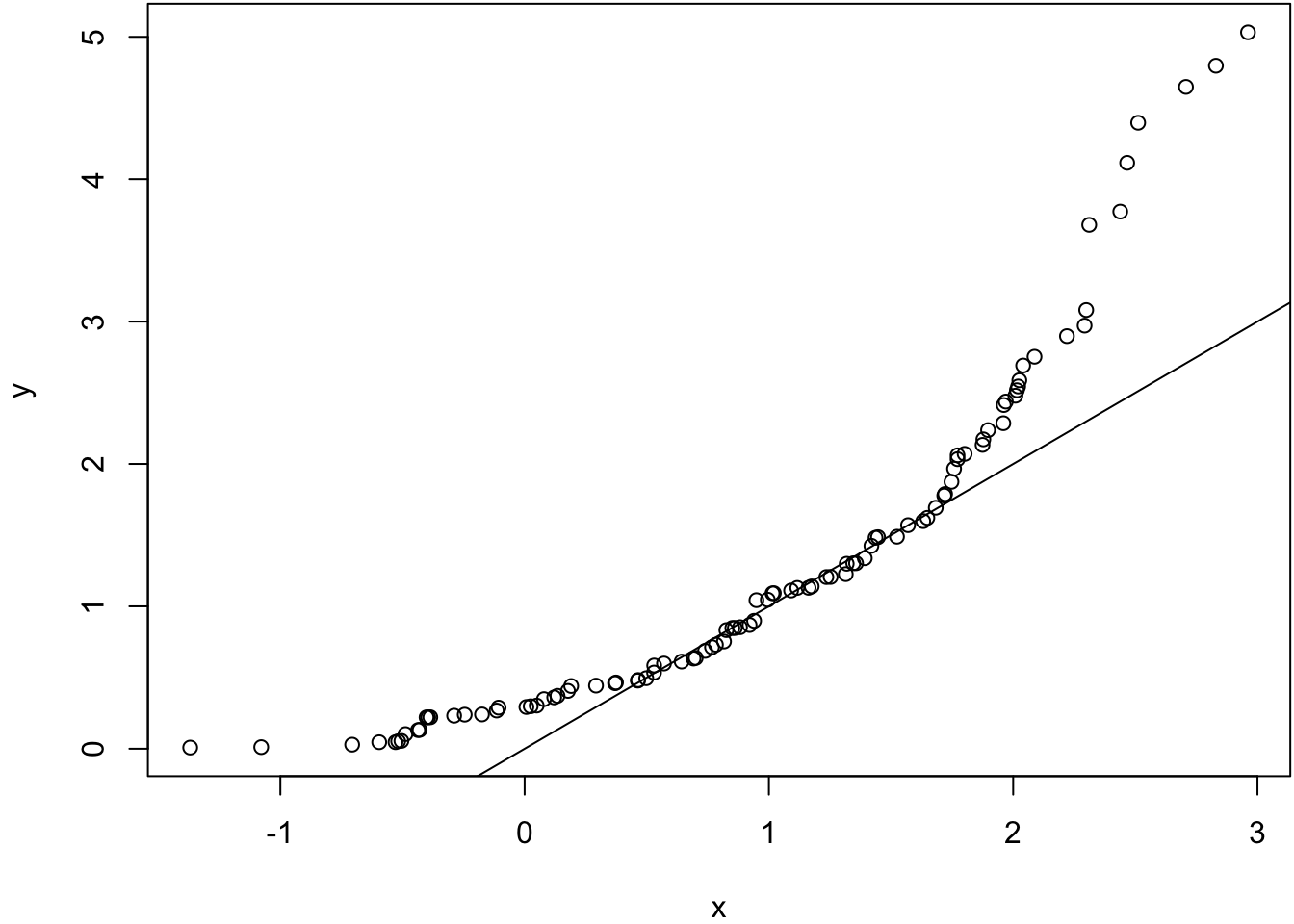
Same population mean and variance. Large sample size.
> x <- rnorm(10000, mean=1)
> y <- rexp(10000, rate=1)
> wilcox.test(x, y)

    Wilcoxon rank sum test with continuity correction

data:  x and y
W = 53311735, p-value = 4.985e-16
alternative hypothesis: true location shift is not equal to 0
> qqplot(x, y); abline(0,1)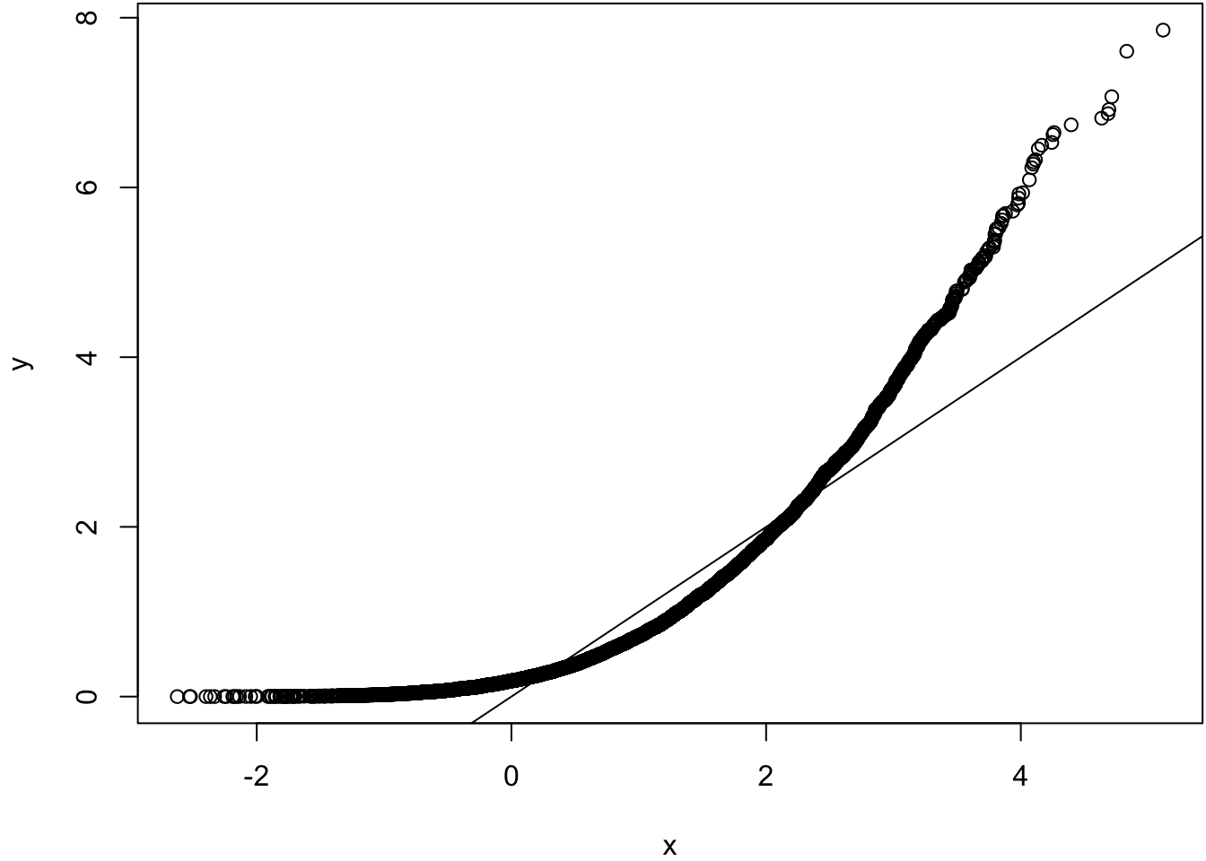
Same mean, very different variances.
> x <- rnorm(100, mean=1, sd=0.01)
> y <- rexp(100, rate=1)
> wilcox.test(x, y)

    Wilcoxon rank sum test with continuity correction

data:  x and y
W = 6579, p-value = 0.0001148
alternative hypothesis: true location shift is not equal to 0
> qqplot(x, y); abline(0,1)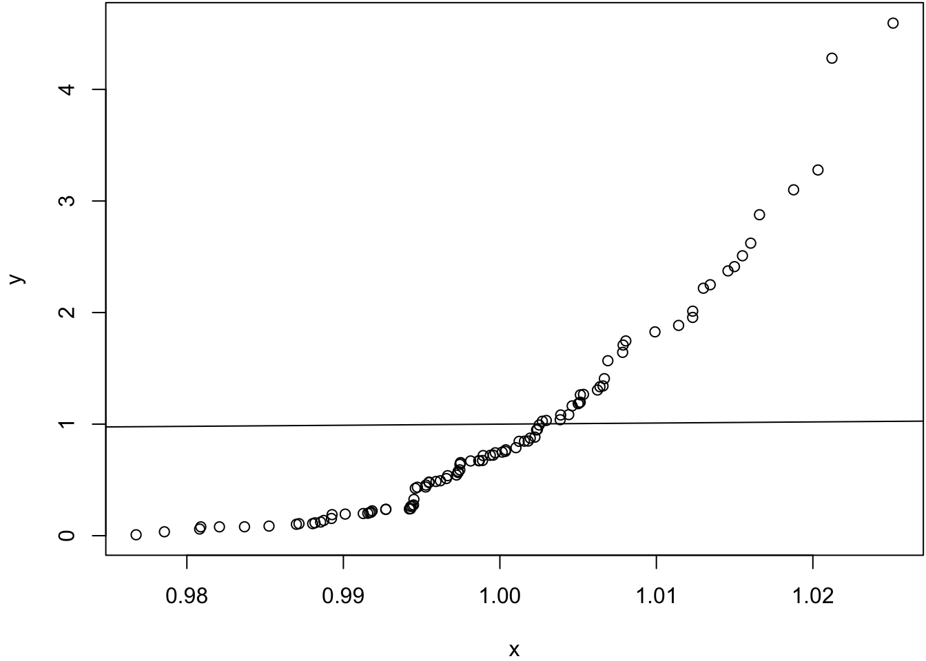
Same variances, different means.
> x <- rnorm(100, mean=2)
> y <- rexp(100, rate=1)
> wilcox.test(x, y)

    Wilcoxon rank sum test with continuity correction

data:  x and y
W = 7836, p-value = 4.261e-12
alternative hypothesis: true location shift is not equal to 0
> qqplot(x, y); abline(0,1)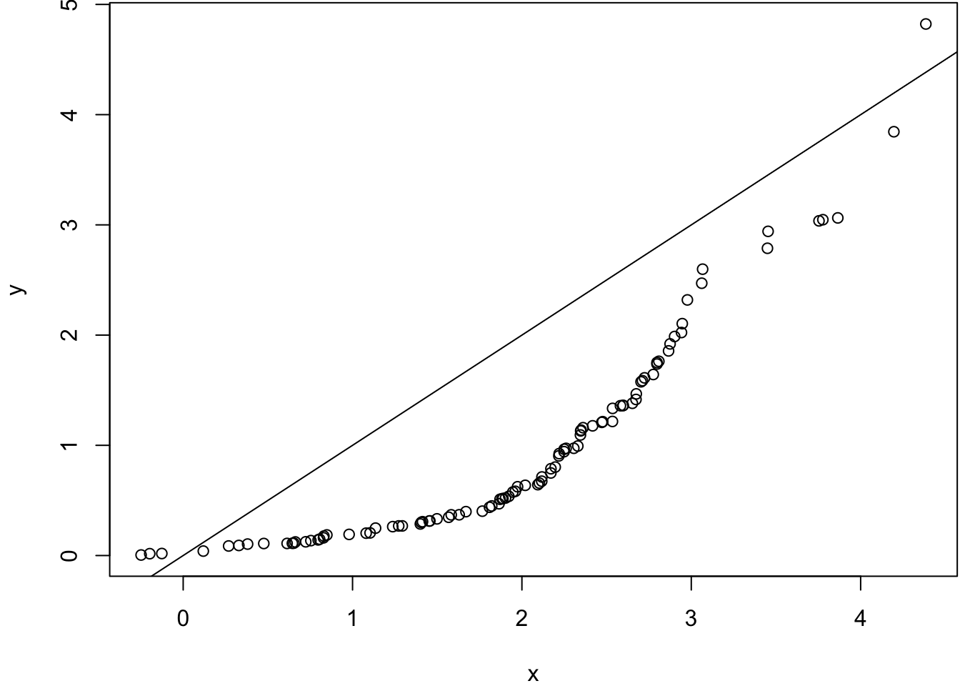
Same population mean and variance.
> x <- rnorm(100, mean=1)
> y <- rexp(100, rate=1)
> wilcox.test(x, y, paired=TRUE)

    Wilcoxon signed rank test with continuity correction

data:  x and y
V = 2394, p-value = 0.6536
alternative hypothesis: true location shift is not equal to 0
> hist(y-x)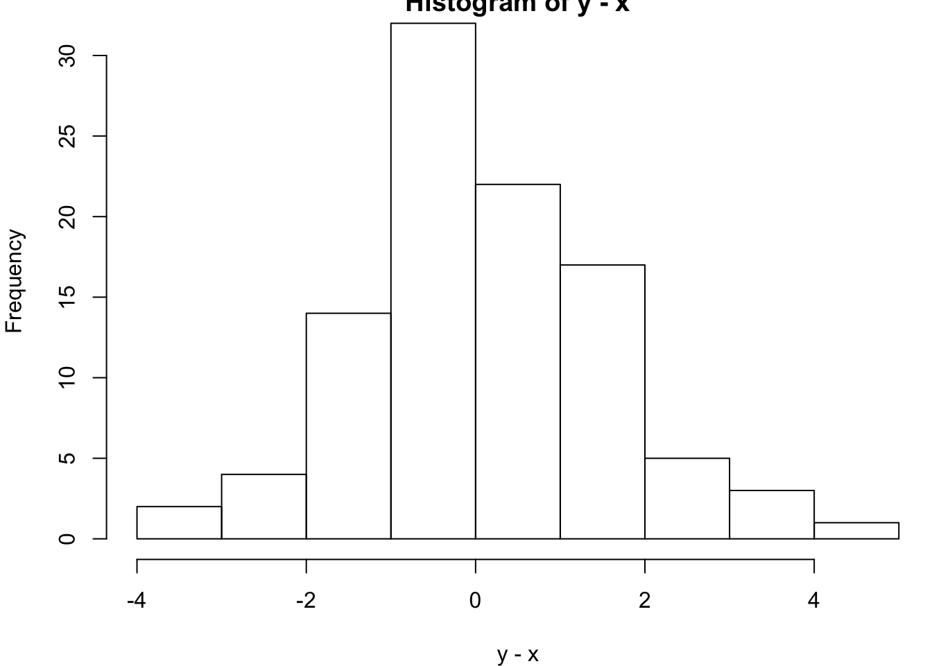
Same population mean and variance. Large sample size.
> x <- rnorm(10000, mean=1)
> y <- rexp(10000, rate=1)
> wilcox.test(x, y, paired=TRUE)

    Wilcoxon signed rank test with continuity correction

data:  x and y
V = 26769956, p-value = 9.23e-10
alternative hypothesis: true location shift is not equal to 0
> hist(y-x)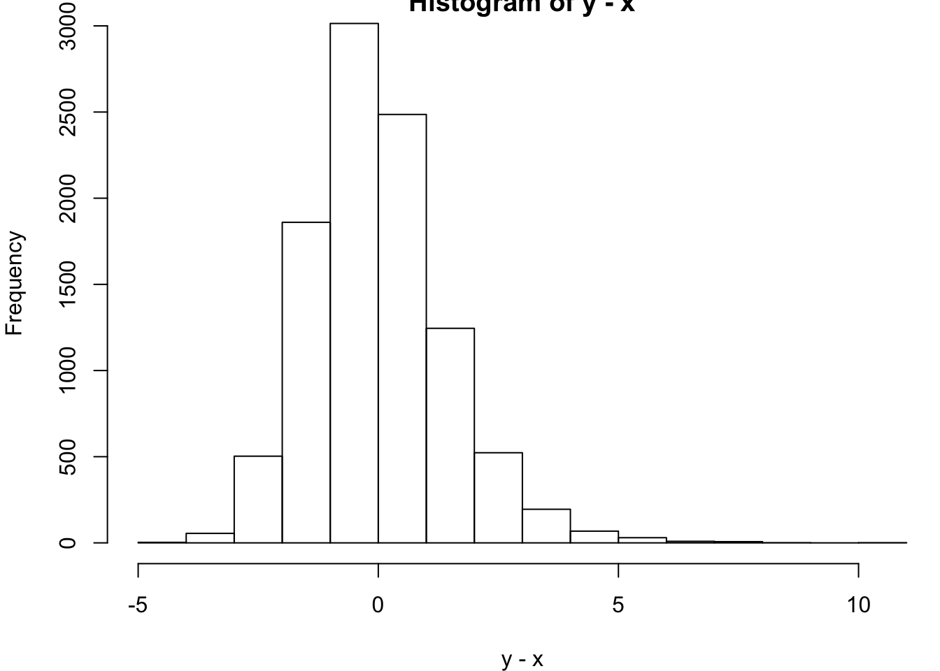
51.6 Permutation t-test
As above, suppose \(X_1, X_2, \ldots, X_m {\; \stackrel{\text{iid}}{\sim}\;}F_X\) and \(Y_1, Y_2, \ldots, Y_n {\; \stackrel{\text{iid}}{\sim}\;}F_Y\), and we wish to test \(H_0: F_X = F_Y\) vs \(H_1: F_X \not= F_Y\). However, suppose we additionally know that \({\operatorname{Var}}(X) = {\operatorname{Var}}(Y)\). We can use a t-statistic to test this hypothesis:
\[ t = \frac{\overline{x} - \overline{y}}{\sqrt{\left(\frac{1}{m} + \frac{1}{n}\right) s^2}} \]
where \(s^2\) is the pooled sample variance.
To obtain the null distribution, we randomly permute the observations to assign \(m\) data points to the \(X\) sample and \(n\) to the \(Y\) sample. This yields permutation data set \(x^{*} = (x_1^{*}, x_2^{*}, \ldots, x_m^{*})^T\) and \(y^{*} = (y_1^{*}, y_2^{*}, \ldots, y_n^{*})^T\). We form null t-statistic
\[ t^{*} = \frac{\overline{x}^{*} - \overline{y}^{*}}{\sqrt{\left(\frac{1}{m} + \frac{1}{n}\right) s^{2*}}} \]
where again \(s^{2*}\) is the pooled sample variance.
In order to obtain a p-value, we calculate \(t^{*(b)}\) for \(b=1, 2, \ldots, B\) permutation data sets.
The p-value of \(t\) is then the proportion of permutation statistics as or more extreme than the observed statistic:
\[ \mbox{p-value}(t) = \frac{1}{B} \sum_{b=1}^{B} 1\left(|t^{*(b)}| \geq |t|\right). \]