66 Generalized Linear Models

66.1 Definition

The generalized linear model (GLM) builds from OLS and GLS to allow for the case where \(Y | {\boldsymbol{X}}\) is distributed according to an exponential family distribution. The estimated model is

\[ g\left({\operatorname{E}}[Y | {\boldsymbol{X}}]\right) = {\boldsymbol{X}}{\boldsymbol{\beta}}\]

where \(g(\cdot)\) is called the link function. This model is typically fit by numerical methods to calculate the maximum likelihood estimate of \({\boldsymbol{\beta}}\).

66.2 Exponential Family Distributions

Recall that if \(Y\) follows an EFD then it has pdf of the form

\[f(y ; \boldsymbol{\theta}) = h(y) \exp \left\{ \sum_{k=1}^d \eta_k(\boldsymbol{\theta}) T_k(y) - A(\boldsymbol{\eta}) \right\} \]

where \(\boldsymbol{\theta}\) is a vector of parameters, \(\{T_k(y)\}\) are sufficient statistics, \(A(\boldsymbol{\eta})\) is the cumulant generating function.

The functions \(\eta_k(\boldsymbol{\theta})\) for \(k=1, \ldots, d\) map the usual parameters \({\boldsymbol{\theta}}\) (often moments of the rv \(Y\)) to the natural parameters or canonical parameters.

\(\{T_k(y)\}\) are sufficient statistics for \(\{\eta_k\}\) due to the factorization theorem.

\(A(\boldsymbol{\eta})\) is sometimes called the log normalizer because

\[A(\boldsymbol{\eta}) = \log \int h(y) \exp \left\{ \sum_{k=1}^d \eta_k(\boldsymbol{\theta}) T_k(y) \right\}.\]

66.3 Natural Single Parameter EFD

A natural single parameter EFD simplifies to the scenario where \(d=1\) and \(T(y) = y\)

\[f(y ; \eta) = h(y) \exp \left\{ \eta(\theta) y - A(\eta(\theta)) \right\} \]

where without loss of generality we can write \({\operatorname{E}}[Y] = \theta\).

66.4 Dispersion EFDs

The family of distributions for which GLMs are most typically developed are dispersion EFDs. An example of a dispersion EFD that extends the natural single parameter EFD is

\[f(y ; \eta) = h(y, \phi) \exp \left\{ \frac{\eta(\theta) y - A(\eta(\theta))}{\phi} \right\} \]

where \(\phi\) is the dispersion parameter.

66.5 Example: Normal

Let \(Y \sim \mbox{Normal}(\mu, \sigma^2)\). Then:

\[ \theta = \mu, \eta(\mu) = \mu \]

\[ \phi = \sigma^2 \]

\[ A(\mu) = \frac{\mu^2}{2} \]

\[ h(y, \sigma^2) = \frac{1}{\sqrt{2\pi\sigma^2}} e^{-\frac{1}{2}\frac{y^2}{\sigma^2}} \]

66.6 EFD for GLMs

There has been a very broad development of GLMs and extensions. A common setting for introducting GLMs is the dispersion EFD with a general link function \(g(\cdot)\).

See the classic text Generalized Linear Models, by McCullagh and Nelder, for such a development.

66.7 Components of a GLM

Random: The particular exponential family distribution. \[ Y \sim f(y ; \eta, \phi) \]
Systematic: The determination of each \(\eta_i\) from \({\boldsymbol{X}}_i\) and \({\boldsymbol{\beta}}\). \[ \eta_i = {\boldsymbol{X}}_i {\boldsymbol{\beta}}\]
Parametric Link: The connection between \(E[Y_i|{\boldsymbol{X}}_i]\) and \({\boldsymbol{X}}_i {\boldsymbol{\beta}}\). \[ g(E[Y_i|{\boldsymbol{X}}_i]) = {\boldsymbol{X}}_i {\boldsymbol{\beta}}\]

66.8 Link Functions

Even though the link function \(g(\cdot)\) can be considered in a fairly general framework, the canonical link function \(\eta(\cdot)\) is often utilized.

The canonical link function is the function that maps the expected value into the natural paramater.

In this case, \(Y | {\boldsymbol{X}}\) is distributed according to an exponential family distribution with

\[ \eta \left({\operatorname{E}}[Y | {\boldsymbol{X}}]\right) = {\boldsymbol{X}}{\boldsymbol{\beta}}. \]

66.9 Calculating MLEs

Given the model \(g\left({\operatorname{E}}[Y | {\boldsymbol{X}}]\right) = {\boldsymbol{X}}{\boldsymbol{\beta}}\), the EFD should be fully parameterized. The Newton-Raphson method or Fisher’s scoring method can be utilized to find the MLE of \({\boldsymbol{\beta}}\).

66.10 Newton-Raphson

Initialize \({\boldsymbol{\beta}}^{(0)}\). For \(t = 1, 2, \ldots\)
Calculate the score \(s({\boldsymbol{\beta}}^{(t)}) = \nabla \ell({\boldsymbol{\beta}}; {\boldsymbol{X}}, {\boldsymbol{Y}}) \mid_{{\boldsymbol{\beta}}= {\boldsymbol{\beta}}^{(t)}}\) and observed Fisher information \[H({\boldsymbol{\beta}}^{(t)}) = - \nabla \nabla^T \ell({\boldsymbol{\beta}}; {\boldsymbol{X}}, {\boldsymbol{Y}}) \mid_{{\boldsymbol{\beta}}= {\boldsymbol{\beta}}^{(t)}}\]. Note that the observed Fisher information is also the negative Hessian matrix.
Update \({\boldsymbol{\beta}}^{(t+1)} = {\boldsymbol{\beta}}^{(t)} + H({\boldsymbol{\beta}}^{(t)})^{-1} s({\boldsymbol{\beta}}^{(t)})\).
Iterate until convergence, and set \(\hat{{\boldsymbol{\beta}}} = {\boldsymbol{\beta}}^{(\infty)}\).

66.11 Fisher’s scoring

Initialize \({\boldsymbol{\beta}}^{(0)}\). For \(t = 1, 2, \ldots\)
Calculate the score \(s({\boldsymbol{\beta}}^{(t)}) = \nabla \ell({\boldsymbol{\beta}}; {\boldsymbol{X}}, {\boldsymbol{Y}}) \mid_{{\boldsymbol{\beta}}= {\boldsymbol{\beta}}^{(t)}}\) and expected Fisher information \[I({\boldsymbol{\beta}}^{(t)}) = - {\operatorname{E}}\left[\nabla \nabla^T \ell({\boldsymbol{\beta}}; {\boldsymbol{X}}, {\boldsymbol{Y}}) \mid_{{\boldsymbol{\beta}}= {\boldsymbol{\beta}}^{(t)}} \right].\]
Update \({\boldsymbol{\beta}}^{(t+1)} = {\boldsymbol{\beta}}^{(t)} + I({\boldsymbol{\beta}}^{(t)})^{-1} s({\boldsymbol{\beta}}^{(t)})\).
Iterate until convergence, and set \(\hat{{\boldsymbol{\beta}}} = {\boldsymbol{\beta}}^{(\infty)}\).

When the canonical link function is used, the Newton-Raphson algorithm and Fisher’s scoring algorithm are equivalent.

Exercise: Prove this.

66.12 Iteratively Reweighted Least Squares

For the canonical link, Fisher’s scoring method can be written as an iteratively reweighted least squares algorithm, as shown earlier for logistic regression. Note that the Fisher information is

\[ I({\boldsymbol{\beta}}^{(t)}) = {\boldsymbol{X}}^T {\boldsymbol{W}}{\boldsymbol{X}}\]

where \({\boldsymbol{W}}\) is an \(n \times n\) diagonal matrix with \((i, i)\) entry equal to \({\operatorname{Var}}(Y_i | {\boldsymbol{X}}; {\boldsymbol{\beta}}^{(t)})\).

The score function is

\[ s({\boldsymbol{\beta}}^{(t)}) = {\boldsymbol{X}}^T \left( {\boldsymbol{Y}}- {\boldsymbol{X}}{\boldsymbol{\beta}}^{(t)} \right) \]

and the current coefficient value \({\boldsymbol{\beta}}^{(t)}\) can be written as

\[ {\boldsymbol{\beta}}^{(t)} = ({\boldsymbol{X}}^T {\boldsymbol{W}}{\boldsymbol{X}})^{-1} {\boldsymbol{X}}^T {\boldsymbol{W}}{\boldsymbol{X}}{\boldsymbol{\beta}}^{(t)}. \]

Putting this together we get

\[ {\boldsymbol{\beta}}^{(t)} + I({\boldsymbol{\beta}}^{(t)})^{-1} s({\boldsymbol{\beta}}^{(t)}) = ({\boldsymbol{X}}^T {\boldsymbol{W}}{\boldsymbol{X}})^{-1} {\boldsymbol{X}}^T {\boldsymbol{W}}{\boldsymbol{z}}^{(t)} \]

where

\[ {\boldsymbol{z}}^{(t)} = {\boldsymbol{X}}{\boldsymbol{\beta}}^{(t)} + {\boldsymbol{W}}^{-1} \left( {\boldsymbol{Y}}- {\boldsymbol{X}}{\boldsymbol{\beta}}^{(t)} \right). \]

This is a generalization of the iteratively reweighted least squares algorithm we showed earlier for logistic regression.

66.13 Estimating Dispersion

For the simple dispersion model above, it is typically straightforward to calculate the MLE \(\hat{\phi}\) once \(\hat{{\boldsymbol{\beta}}}\) has been calculated.

66.14 CLT Applied to the MLE

Given that \(\hat{{\boldsymbol{\beta}}}\) is a maximum likelihood estimate, we have the following CLT result on its distribution as \(n \rightarrow \infty\):

\[ \sqrt{n} (\hat{{\boldsymbol{\beta}}} - {\boldsymbol{\beta}}) \stackrel{D}{\longrightarrow} \mbox{MVN}_{p}({\boldsymbol{0}}, \phi ({\boldsymbol{X}}^T {\boldsymbol{W}}{\boldsymbol{X}})^{-1}) \]

66.15 Approximately Pivotal Statistics

The previous CLT gives us the following two approximations for pivtoal statistics. The first statistic facilitates getting overall measures of uncertainty on the estimate \(\hat{{\boldsymbol{\beta}}}\).

\[ \hat{\phi}^{-1} (\hat{{\boldsymbol{\beta}}} - {\boldsymbol{\beta}})^T ({\boldsymbol{X}}^T \hat{{\boldsymbol{W}}} {\boldsymbol{X}}) (\hat{{\boldsymbol{\beta}}} - {\boldsymbol{\beta}}) {\; \stackrel{.}{\sim}\;}\chi^2_1 \]

This second pivotal statistic allows for performing a Wald test or forming a confidence interval on each coefficient, \(\beta_j\), for \(j=1, \ldots, p\).

\[ \frac{\hat{\beta}_j - \beta_j}{\sqrt{\hat{\phi} [({\boldsymbol{X}}^T \hat{{\boldsymbol{W}}} {\boldsymbol{X}})^{-1}]_{jj}}} {\; \stackrel{.}{\sim}\;}\mbox{Normal}(0,1) \]

66.16 Deviance

Let \(\hat{\boldsymbol{\eta}}\) be the estimated natural parameters from a GLM. For example, \(\hat{\boldsymbol{\eta}} = {\boldsymbol{X}}\hat{{\boldsymbol{\beta}}}\) when the canonical link function is used.

Let \(\hat{\boldsymbol{\eta}}_n\) be the saturated model wwhere \(Y_i\) is directly used to estimate \(\eta_i\) without model constraints. For example, in the Bernoulli logistic regression model \(\hat{\boldsymbol{\eta}}_n = {\boldsymbol{Y}}\), the observed outcomes.

The deviance for the model is defined to be

\[ D\left(\hat{\boldsymbol{\eta}}\right) = 2 \ell(\hat{\boldsymbol{\eta}}_n; {\boldsymbol{X}}, {\boldsymbol{Y}}) - 2 \ell(\hat{\boldsymbol{\eta}}; {\boldsymbol{X}}, {\boldsymbol{Y}}) \]

66.17 Generalized LRT

Let \({\boldsymbol{X}}_0\) be a subset of \(p_0\) columns of \({\boldsymbol{X}}\) and let \({\boldsymbol{X}}_1\) be a subset of \(p_1\) columns, where \(1 \leq p_0 < p_1 \leq p\). Also, assume that the columns of \({\boldsymbol{X}}_0\) are a subset of \({\boldsymbol{X}}_1\).

Without loss of generality, suppose that \({\boldsymbol{\beta}}_0 = (\beta_1, \beta_2, \ldots, \beta_{p_0})^T\) and \({\boldsymbol{\beta}}_1 = (\beta_1, \beta_2, \ldots, \beta_{p_1})^T\).

Suppose we wish to test \(H_0: (\beta_{p_0+1}, \beta_{p_0 + 2}, \ldots, \beta_{p_1}) = {\boldsymbol{0}}\) vs \(H_1: (\beta_{p_0+1}, \beta_{p_0 + 2}, \ldots, \beta_{p_1}) \not= {\boldsymbol{0}}\)

We can form \(\hat{\boldsymbol{\eta}}_0 = {\boldsymbol{X}}\hat{{\boldsymbol{\beta}}}_0\) from the GLM model \(g\left({\operatorname{E}}[Y | {\boldsymbol{X}}_0]\right) = {\boldsymbol{X}}_0 {\boldsymbol{\beta}}_0\). We can analogously form \(\hat{\boldsymbol{\eta}}_1 = {\boldsymbol{X}}\hat{{\boldsymbol{\beta}}}_1\) from the GLM model \(g\left({\operatorname{E}}[Y | {\boldsymbol{X}}_1]\right) = {\boldsymbol{X}}_1 {\boldsymbol{\beta}}_1\).

The \(2\log\) generalized LRT can then be formed from the two deviance statistics

\[ 2 \log \lambda({\boldsymbol{X}}, {\boldsymbol{Y}}) = 2 \log \frac{L(\hat{\boldsymbol{\eta}}_1; {\boldsymbol{X}}, {\boldsymbol{Y}})}{L(\hat{\boldsymbol{\eta}}_0; {\boldsymbol{X}}, {\boldsymbol{Y}})} = D\left(\hat{\boldsymbol{\eta}}_0\right) - D\left(\hat{\boldsymbol{\eta}}_1\right) \]

where the null distribution is \(\chi^2_{p_1-p_0}\).

66.18 Example: Grad School Admissions

Let’s revisit a logistic regression example now that we know how the various statistics are calculated.

> mydata <- 
+   read.csv("http://www.ats.ucla.edu/stat/data/binary.csv")
> dim(mydata)
> head(mydata)

Fit the model with basic output. Note the argument family = "binomial".

> mydata$rank <- factor(mydata$rank, levels=c(1, 2, 3, 4))
> myfit <- glm(admit ~ gre + gpa + rank, 
+              data = mydata, family = "binomial")
> myfit

Call:  glm(formula = admit ~ gre + gpa + rank, family = "binomial", 
    data = mydata)

Coefficients:
(Intercept)          gre          gpa        rank2        rank3  
  -3.989979     0.002264     0.804038    -0.675443    -1.340204  
      rank4  
  -1.551464  

Degrees of Freedom: 399 Total (i.e. Null);  394 Residual
Null Deviance:      500 
Residual Deviance: 458.5    AIC: 470.5

This shows the fitted coefficient values, which is on the link function scale – logit aka log odds here. Also, a Wald test is performed for each coefficient.

> summary(myfit)

Call:
glm(formula = admit ~ gre + gpa + rank, family = "binomial", 
    data = mydata)

Deviance Residuals: 
    Min       1Q   Median       3Q      Max  
-1.6268  -0.8662  -0.6388   1.1490   2.0790  

Coefficients:
             Estimate Std. Error z value Pr(>|z|)    
(Intercept) -3.989979   1.139951  -3.500 0.000465 ***
gre          0.002264   0.001094   2.070 0.038465 *  
gpa          0.804038   0.331819   2.423 0.015388 *  
rank2       -0.675443   0.316490  -2.134 0.032829 *  
rank3       -1.340204   0.345306  -3.881 0.000104 ***
rank4       -1.551464   0.417832  -3.713 0.000205 ***
---
Signif. codes:  0 '***' 0.001 '**' 0.01 '*' 0.05 '.' 0.1 ' ' 1

(Dispersion parameter for binomial family taken to be 1)

    Null deviance: 499.98  on 399  degrees of freedom
Residual deviance: 458.52  on 394  degrees of freedom
AIC: 470.52

Number of Fisher Scoring iterations: 4

Here we perform a generalized LRT on each variable. Note the rank variable is now tested as a single factor variable as opposed to each dummy variable.

> anova(myfit, test="LRT")
Analysis of Deviance Table

Model: binomial, link: logit

Response: admit

Terms added sequentially (first to last)

     Df Deviance Resid. Df Resid. Dev  Pr(>Chi)    
NULL                   399     499.98              
gre   1  13.9204       398     486.06 0.0001907 ***
gpa   1   5.7122       397     480.34 0.0168478 *  
rank  3  21.8265       394     458.52 7.088e-05 ***
---
Signif. codes:  0 '***' 0.001 '**' 0.01 '*' 0.05 '.' 0.1 ' ' 1

> mydata <- data.frame(mydata, probs = myfit$fitted.values)
> ggplot(mydata) + geom_point(aes(x=gpa, y=probs, color=rank)) +
+   geom_jitter(aes(x=gpa, y=admit), width=0, height=0.01, alpha=0.3)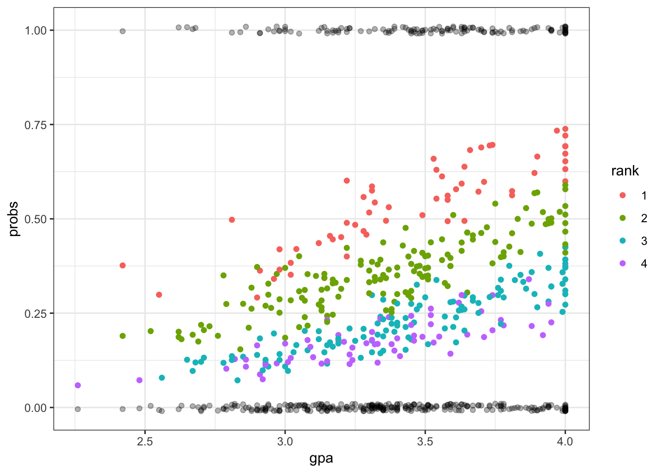

> ggplot(mydata) + geom_point(aes(x=gre, y=probs, color=rank)) +
+   geom_jitter(aes(x=gre, y=admit), width=0, height=0.01, alpha=0.3)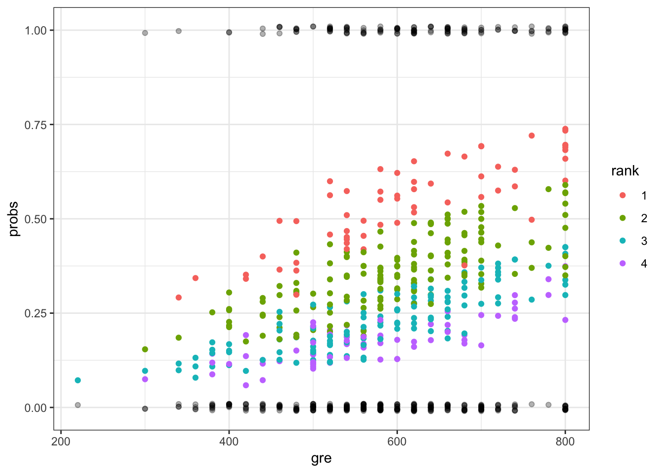

> ggplot(mydata) + geom_boxplot(aes(x=rank, y=probs)) +
+   geom_jitter(aes(x=rank, y=probs), width=0.1, height=0.01, alpha=0.3)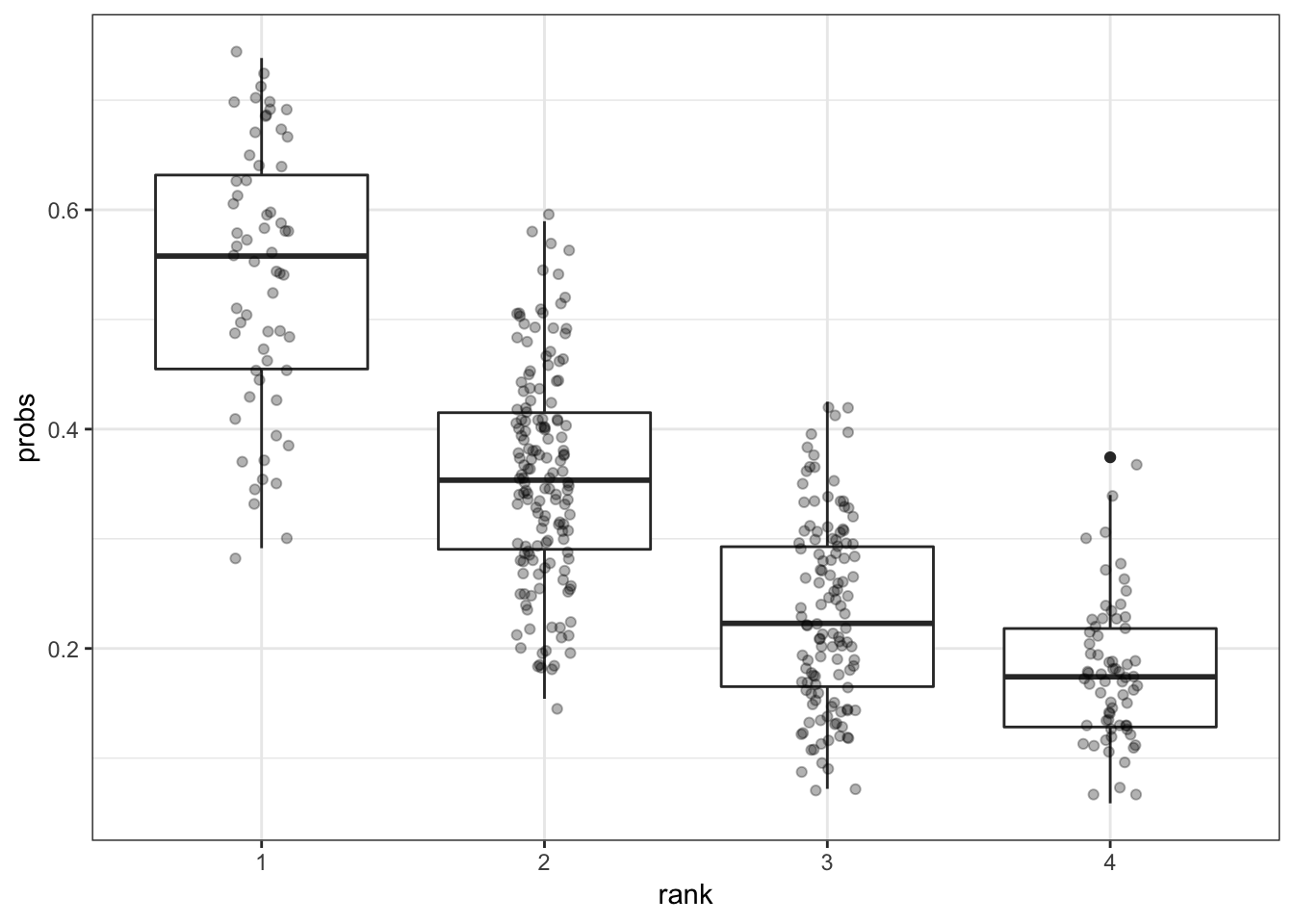

66.19 `glm()` Function

The glm() function has many different options available to the user.

glm(formula, family = gaussian, data, weights, subset,
    na.action, start = NULL, etastart, mustart, offset,
    control = list(...), model = TRUE, method = "glm.fit",
    x = FALSE, y = TRUE, contrasts = NULL, ...)

To see the different link functions available, type:

help(family)