67 Nonparametric Regression
67.1 Simple Linear Regression
Recall the set up for simple linear regression. For random variables \((X_1, Y_1), (X_2, Y_2), \ldots, (X_n, Y_n)\), simple linear regression estimates the model
\[ Y_i = \beta_1 + \beta_2 X_i + E_i \]
where \({\operatorname{E}}[E_i | X_i] = 0\), \({\operatorname{Var}}(E_i | X_i) = \sigma^2\), and \({\operatorname{Cov}}(E_i, E_j | X_i, X_j) = 0\) for all \(1 \leq i, j \leq n\) and \(i \not= j\).
Note that in this model \({\operatorname{E}}[Y | X] = \beta_1 + \beta_2 X.\)
67.2 Simple Nonparametric Regression
In simple nonparametric regression, we define a similar model while eliminating the linear assumption:
\[ Y_i = s(X_i) + E_i \]
for some function \(s(\cdot)\) with the same assumptions on the distribution of \({\boldsymbol{E}}| {\boldsymbol{X}}\). In this model, we also have
\[ {\operatorname{E}}[Y | X] = s(X). \]
67.3 Smooth Functions
Suppose we consider fitting the model \(Y_i = s(X_i) + E_i\) with the restriction that \(s \in C^2\), the class of functions with continuous second derivatives. We can set up an objective function that regularizes how smooth vs wiggly \(s\) is.
Specifically, suppose for a given set of observed data \((x_1, y_1), (x_2, y_2), \ldots, (x_n, y_n)\) we wish to identify a function \(s \in C^2\) that minimizes for some \(\lambda\)
\[ \sum_{i=1}^n (y_i - s(x_i))^2 + \lambda \int |s''(x)|^2 dx \]
67.4 Smoothness Parameter \(\lambda\)
When minimizing
\[ \sum_{i=1}^n (y_i - s(x_i))^2 + \lambda \int |s^{\prime\prime}(x)|^2 dx \]
it follows that if \(\lambda=0\) then any function \(s \in C^2\) that interpolates the data is a solution.
As \(\lambda \rightarrow \infty\), then the minimizing function is the simple linear regression solution.
67.5 The Solution
For an observed data set \((x_1, y_1), (x_2, y_2), \ldots, (x_n, y_n)\) where \(n \geq 4\) and a fixed value \(\lambda\), there is an exact solution to minimizing
\[ \sum_{i=1}^n (y_i - s(x_i))^2 + \lambda \int |s^{\prime\prime}(x)|^2 dx. \]
The solution is called a natural cubic spline, which is constructed to have knots at \(x_1, x_2, \ldots, x_n\).
67.6 Natural Cubic Splines
Suppose without loss of generality that we have ordered \(x_1 < x_2 < \cdots < x_n\). We assume all \(x_i\) are unique to simplify the explanation here, but ties can be deal with.
A natural cubic spline (NCS) is a function constructed from a set of piecewise cubic functions over the range \([x_1, x_n]\) joined at the knots so that the second derivative is continuous at the knots. Outside of the range (\(< x_1\) or \(> x_n\)), the spline is linear and it has continuous second derivatives at the endpoint knots.
67.7 Basis Functions
Depending on the value \(\lambda\), a different ncs will be constructed, but the entire family of ncs solutions over \(0 < \lambda < \infty\) can be constructed from a common set of basis functions.
We construct \(n\) basis functions \(N_1(x), N_2(x), \ldots, N_n(x)\) with coefficients \(\theta_1(\lambda), \theta_2(\lambda), \ldots, \theta_n(\lambda)\). The NCS takes the form
\[ s(x) = \sum_{i=1}^n \theta_i(\lambda) N_i(x). \]
Define \(N_1(x) = 1\) and \(N_2(x) = x\). For \(i = 3, \ldots, n\), define \(N_i(x) = d_{i-1}(x) - d_{i-2}(x)\) where
\[ d_{i}(x) = \frac{(x - x_i)^3 - (x - x_n)^3}{x_n - x_i}. \]
Recall that we’ve labeled indices so that \(x_1 < x_2 < \cdots < x_n\).
67.8 Calculating the Solution
Let \({\boldsymbol{\theta}}_\lambda = (\theta_1(\lambda), \theta_2(\lambda), \ldots, \theta_n(\lambda))^T\) and let \({\boldsymbol{N}}\) be the \(n \times n\) matrix with \((i, j)\) entry equal to \(N_j(x_i)\). Finally, let \({\boldsymbol{\Omega}}\) be the \(n \times n\) matrix with \((i,j)\) entry equal to \(\int N_i^{\prime\prime}(x) N_j^{\prime\prime}(x) dx\).
The solution to \({\boldsymbol{\theta}}_\lambda\) are the values that minimize
\[ ({\boldsymbol{y}}- {\boldsymbol{N}}{\boldsymbol{\theta}})^T ({\boldsymbol{y}}- {\boldsymbol{N}}{\boldsymbol{\theta}}) + \lambda {\boldsymbol{\theta}}^T {\boldsymbol{\Omega}}{\boldsymbol{\theta}}. \]
which results in
\[ \hat{{\boldsymbol{\theta}}}_\lambda = ({\boldsymbol{N}}^T {\boldsymbol{N}}+ \lambda {\boldsymbol{\Omega}})^{-1} {\boldsymbol{N}}^T {\boldsymbol{y}}. \]
67.9 Linear Operator
Letting
\[ {\boldsymbol{S}}_\lambda = {\boldsymbol{N}}({\boldsymbol{N}}^T {\boldsymbol{N}}+ \lambda {\boldsymbol{\Omega}})^{-1} {\boldsymbol{N}}^T \]
it folows that the fitted values are
\[ \hat{{\boldsymbol{y}}} = {\boldsymbol{S}}_\lambda {\boldsymbol{y}}. \]
Thus, the fitted values from a NCS are contructed by taking linear combination of the response variable values \(y_1, y_2, \ldots, y_n\).
67.10 Degrees of Freedom
Recall that in OLS, we formed projection matrix \({\boldsymbol{P}}= {\boldsymbol{X}}({\boldsymbol{X}}^T {\boldsymbol{X}})^{-1} {\boldsymbol{X}}^T\) and noted that the number of columns \(p\) of \({\boldsymbol{X}}\) is also found in the trace of \({\boldsymbol{P}}\) where \(\operatorname{tr}({\boldsymbol{P}}) = p\).
The effective degrees of freedom for a model fit by a linear operator is calculated as the trace of the operator.
Therefore, for a given \(\lambda\), the effective degrees of freedom is
\[ \operatorname{df}_\lambda = \operatorname{tr}({\boldsymbol{S}}_\lambda). \]
67.11 Bayesian Intepretation
Minimizing
\[ \sum_{i=1}^n (y_i - s(x_i))^2 + \lambda \int |s^{\prime\prime}(x)|^2 dx \]
is equivalent to maximizing
\[ \exp\left\{ -\frac{\sum_{i=1}^n (y_i - s(x_i))^2}{2\sigma^2} \right\} \exp\left\{-\frac{\lambda}{2\sigma^2} \int |s^{\prime\prime}(x)|^2 dx\right\}. \]
Therefore, the NCS solution can be interpreted as calculting the MAP where \(Y | X\) is Normal and there’s an Exponential prior on the smoothness of \(s\).
67.12 Bias and Variance Trade-off
Typically we will choose some \(0 < \lambda < \infty\) in an effort to balance the bias and variance. Let \(\hat{Y} = \hat{s}(X; \lambda)\) where \(\hat{s}(\cdot; \lambda)\) minimizes the above for some chosen \(\lambda\) on an independent data set. Then
\[ \begin{aligned} {\operatorname{E}}\left[\left(Y - \hat{Y}\right)^2\right] & = {\rm E}\left[\left(s(x) + E - \hat{s}(x; \lambda)\right)^2 \right] \\ \ & = {\rm E}\left[\left( s(x) - \hat{s}(x; \lambda) \right)^2 \right] + {\rm Var}(E) \\ \ & = \left( s(x) - {\rm E}[\hat{s}(x; \lambda)]\right)^2 + {\rm Var}\left(\hat{s}(x; \lambda)\right) + {\rm Var}(E) \\ \ & = \mbox{bias}^2_{\lambda} + \mbox{variance}_{\lambda} + {\rm Var}(E) \end{aligned} \]
where all of the above calculations are conditioned on \(X=x\).
In minimizing
\[ \sum_{i=1}^n (y_i - s(x_i))^2 + \lambda \int |s^{\prime\prime}(x)|^2 dx \]
the relationship is such that:
\[ \uparrow \lambda \Longrightarrow \mbox{bias}^2 \uparrow, \mbox{variance} \downarrow \]
\[ \downarrow \lambda \Longrightarrow \mbox{bias}^2 \downarrow, \mbox{variance} \uparrow \]
67.13 Choosing \(\lambda\)
There are several approaches that are commonly used to identify a value of \(\lambda\), including:
- Scientific knowledge that guides the acceptable value of \(\operatorname{df}_\lambda\)
- Cross-validation or some other prediction quality measure
- Model selection measures, such as Akaike information criterion (AIC) or Mallows \(C_p\)
67.14 Smoothers and Spline Models
We investigated one type of nonparametric regression model here, the NCS. However, in general there are many such “smoother” methods available in the simple nonparametric regression scenario.
Splines are particularly popular since splines are constructed from putting together polynomials and are therefore usually tractable to compute and analyze.
67.15 Smoothers in R
There are several functions and packages available in R for computing smoothers and tuning smoothness parameters. Examples include:
splineslibrarysmooth.spline()loess()lowess()
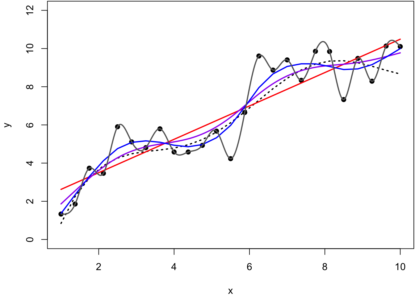
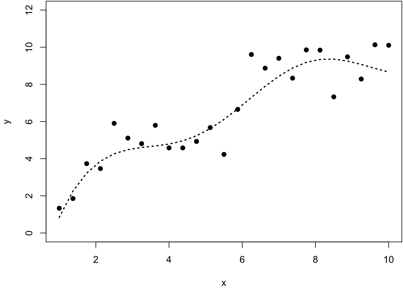
67.16 Example
> y2 <- smooth.spline(x=x, y=y, df=2)
> y5 <- smooth.spline(x=x, y=y, df=5)
> y25 <- smooth.spline(x=x, y=y, df=25)
> ycv <- smooth.spline(x=x, y=y)
> ycv
Call:
smooth.spline(x = x, y = y)

Smoothing Parameter  spar= 0.5162045  lambda= 0.0002730906 (11 iterations)
Equivalent Degrees of Freedom (Df): 7.293673
Penalized Criterion (RSS): 14.80602
GCV: 1.180651