79 Surrogate Variable Analysis
The surrogate variable analysis (SVA) model combines the many responses model with the latent variable model introduced above:
\[ {\boldsymbol{Y}}_{m \times n} = {\boldsymbol{B}}_{m \times d} {\boldsymbol{X}}_{d \times n} + {\boldsymbol{\Phi}}_{m \times r} {\boldsymbol{Z}}_{r \times n} + {\boldsymbol{E}}_{m \times n} \]
where \(m \gg n > d + r\).
Here, only \({\boldsymbol{Y}}\) and \({\boldsymbol{X}}\) are observed, so we must combine many regressors model fitting techniques with latent variable estimation.
The variables \({\boldsymbol{Z}}\) are called surrogate variables for what would be a complete model of all systematic variation.
79.1 Procedure
The main challenge is that the row spaces of \({\boldsymbol{X}}\) and \({\boldsymbol{Z}}\) may overlap. Even when \({\boldsymbol{X}}\) is the result of a randomized experiment, there will be a high probability that the row spaces of \({\boldsymbol{X}}\) and \({\boldsymbol{Z}}\) have some overlap.
Therefore, one cannot simply estimate \({\boldsymbol{Z}}\) by applying a latent variable esitmation method on the residuals \({\boldsymbol{Y}}- \hat{{\boldsymbol{B}}} {\boldsymbol{X}}\) or on the observed response data \({\boldsymbol{Y}}\). In the former case, we will only estimate \({\boldsymbol{Z}}\) in the space orthogonal to \(\hat{{\boldsymbol{B}}} {\boldsymbol{X}}\). In the latter case, the estimate of \({\boldsymbol{Z}}\) may modify the signal we can estimate in \({\boldsymbol{B}}{\boldsymbol{X}}\).
A recent method, takes an EM approach to esitmating \({\boldsymbol{Z}}\) in the model
\[ {\boldsymbol{Y}}_{m \times n} = {\boldsymbol{B}}_{m \times d} {\boldsymbol{X}}_{d \times n} + {\boldsymbol{\Phi}}_{m \times r} {\boldsymbol{Z}}_{r \times n} + {\boldsymbol{E}}_{m \times n}. \]
It is shown to be necessary to penalize the likelihood in the estimation of \({\boldsymbol{B}}\) — i.e., form shrinkage estimates of \({\boldsymbol{B}}\) — in order to properly balance the row spaces of \({\boldsymbol{X}}\) and \({\boldsymbol{Z}}\).
The regularized EM algorithm, called cross-dimensonal inference (CDI) iterates between
- Estimate \({\boldsymbol{Z}}\) from \({\boldsymbol{Y}}- \hat{{\boldsymbol{B}}}^{\text{Reg}} {\boldsymbol{X}}\)
- Estimate \({\boldsymbol{B}}\) from \({\boldsymbol{Y}}- \hat{{\boldsymbol{\Phi}}} \hat{{\boldsymbol{Z}}}\)
where \(\hat{{\boldsymbol{B}}}^{\text{Reg}}\) is a regularized or shrunken estimate of \({\boldsymbol{B}}\).
It can be shown that when the regularization can be represented by a prior distribution on \({\boldsymbol{B}}\) then this algorithm achieves the MAP.
79.2 Example: Kidney Expr by Age
In Storey et al. (2005), we considered a study where kidney samples were obtained on individuals across a range of ages. The goal was to identify genes with expression associated with age.
> library(edge)
> library(splines)
> load("./data/kidney.RData")
> age <- kidcov$age
> sex <- kidcov$sex
> dim(kidexpr)
[1] 34061    72
> cov <- data.frame(sex = sex, age = age)
> null_model <- ~sex
> full_model <- ~sex + ns(age, df = 3)
> de_obj <- build_models(data = kidexpr, cov = cov,
+ null.model = null_model,
+ full.model = full_model)
> de_lrt <- lrt(de_obj, nullDistn = "bootstrap", bs.its = 100, verbose=FALSE)
> qobj1 <- qvalueObj(de_lrt)
> hist(qobj1)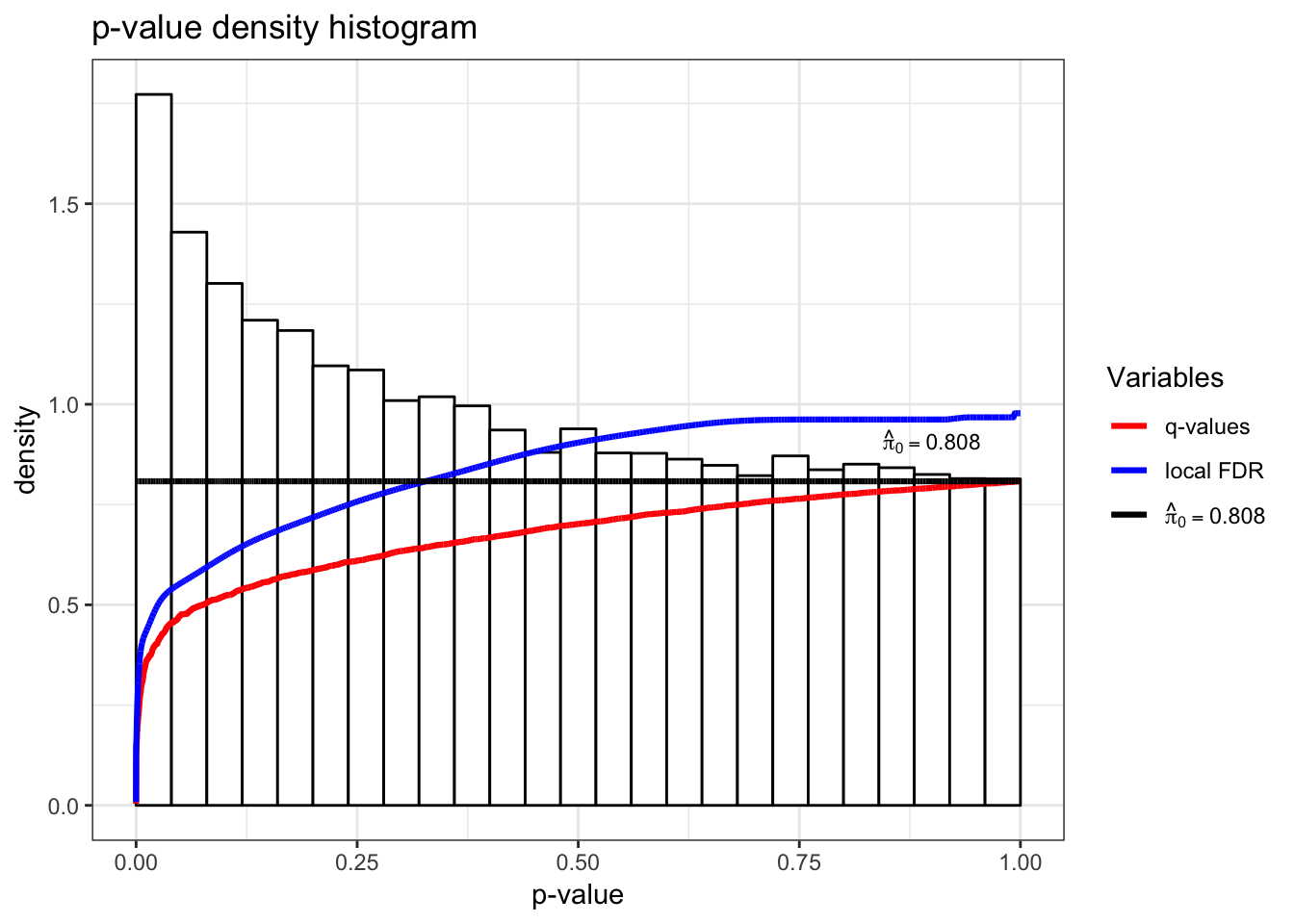
Now that we have completed a standard generalized LRT, let’s estimate \({\boldsymbol{Z}}\) (the surrogate variables) using the sva package as accessed via the edge package.
> dim(nullMatrix(de_obj))
[1] 72  2
> de_sva <- apply_sva(de_obj, n.sv=4, method="irw", B=10)
Number of significant surrogate variables is:  4
Iteration (out of 10 ):1  2  3  4  5  6  7  8  9  10
> dim(nullMatrix(de_sva))
[1] 72  6
> de_svalrt <- lrt(de_sva, nullDistn = "bootstrap", bs.its = 100, verbose=FALSE)
> qobj2 <- qvalueObj(de_svalrt)
> hist(qobj2)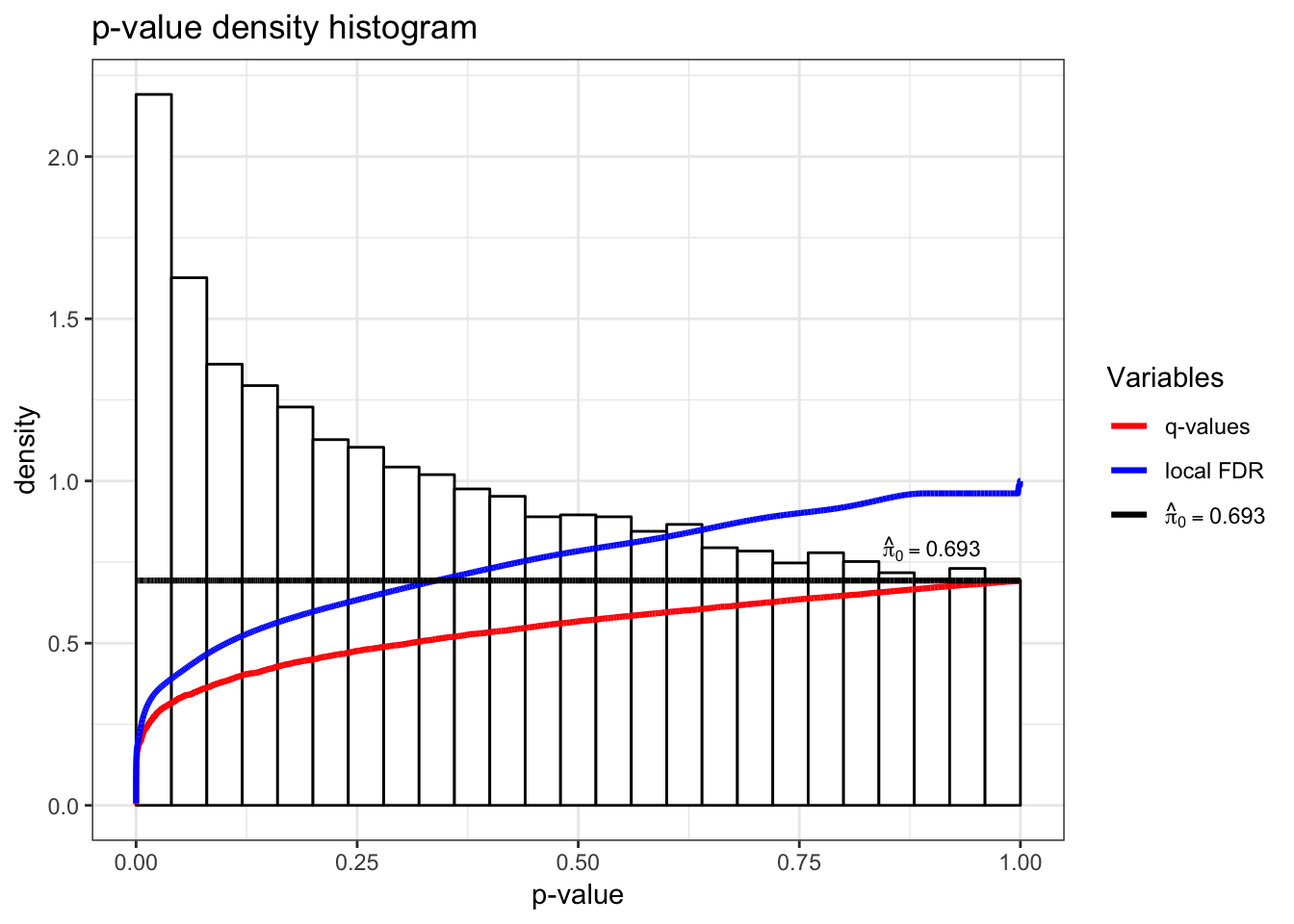
> summary(qobj1)

Call:
qvalue(p = pval)

pi0:    0.8081212

Cumulative number of significant calls:

          <1e-04 <0.001 <0.01 <0.025 <0.05 <0.1    <1
p-value       27    161   798   1676  2906 5271 34061
q-value        0      0     2      4    10   27 34061
local FDR      0      0     2      2     5   18 34061
> summary(qobj2)
Call:
qvalue(p = pval)
pi0: 0.6925105
Cumulative number of significant calls:
<1e-04 <0.001 <0.01 <0.025 <0.05 <0.1 <1
p-value 28 151 1001 2051 3549 6168 34061
q-value 0 0 3 4 6 51 34061
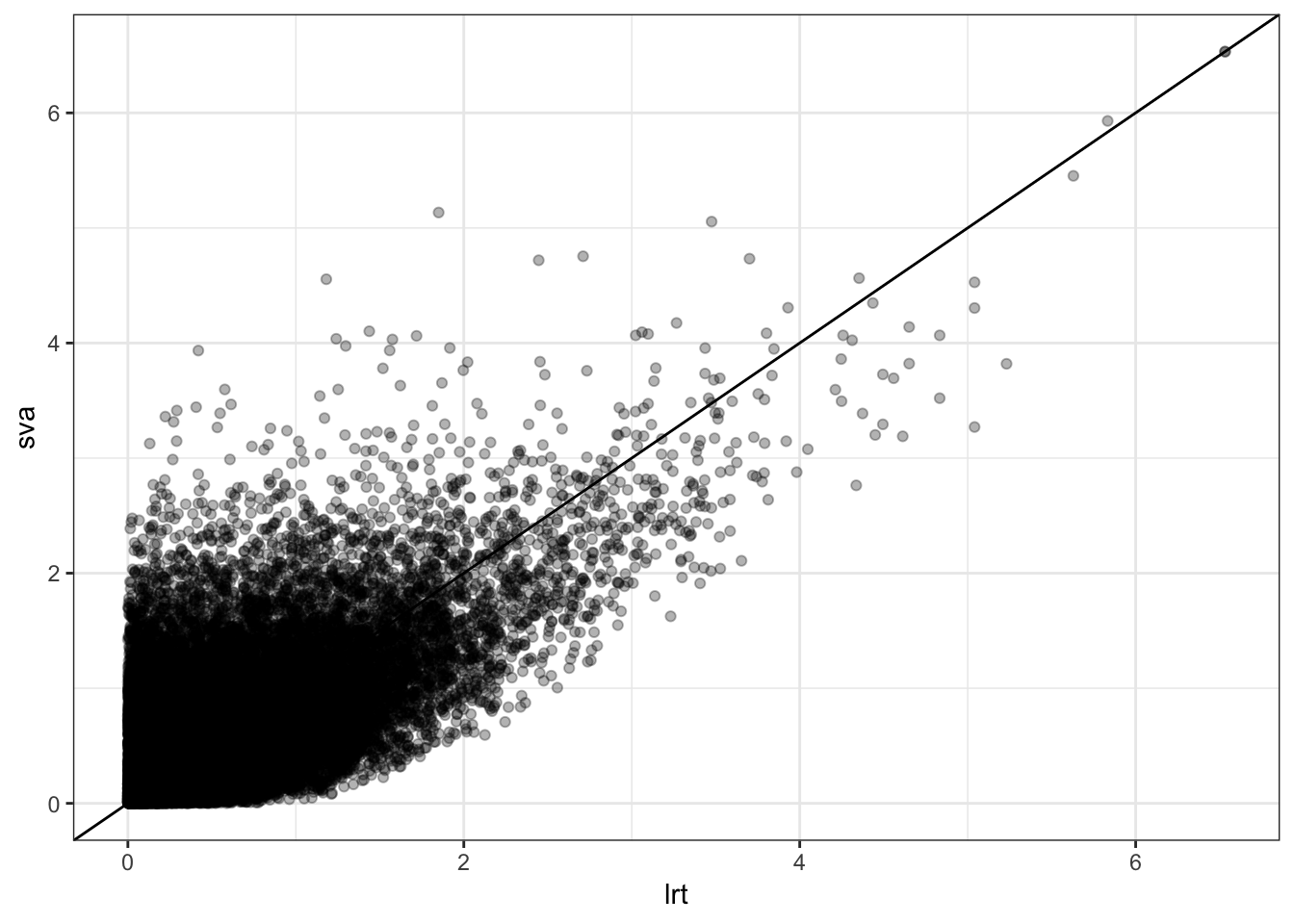
local FDR 0 0 2 2 3 28 34053P-values from two analyses are fairly different.
> data.frame(lrt=-log10(qobj1$pval), sva=-log10(qobj2$pval)) %>%
+   ggplot() + geom_point(aes(x=lrt, y=sva), alpha=0.3) + geom_abline()