18 Convergence of Random Variables
18.1 Sequence of RVs
Let \(Z_1, Z_2, \ldots\) be an infinite sequence of rv’s.
An important example is
\[Z_n = \overline{X}_n = \frac{\sum_{i=1}^n X_i}{n}.\]
It is useful to be able to determine a limiting value or distribution of \(\{Z_i\}\).
18.2 Convergence in Distribution
\(\{Z_i\}\) converges in distribution to \(Z\), written
\[Z_n \stackrel{D}{\longrightarrow} Z\]
if
\[F_{Z_n}(y) = \Pr(Z_n \leq y) \rightarrow \Pr(Z \leq y) = F_{Z}(y)\]
as \(n \rightarrow \infty\) for all \(y \in \mathbb{R}\).
18.3 Convergence in Probability
\(\{Z_i\}\) converges in probability to \(Z\), written
\[Z_n \stackrel{P}{\longrightarrow} Z\]
if
\[\Pr(|Z_n - Z| \leq \epsilon) \rightarrow 1\]
as \(n \rightarrow \infty\) for all \(\epsilon > 0\).
Note that it may also be the case that \(Z_n \stackrel{P}{\longrightarrow} \theta\) for a fixed, nonrandom value \(\theta\).
18.4 Almost Sure Convergence
\(\{Z_i\}\) converges almost surely (or “with probability 1”) to \(Z\), written
\[Z_n \stackrel{a.s.}{\longrightarrow} Z\]
if
\[\Pr\left(\{\omega: |Z_n(\omega) - Z(\omega)| \stackrel{n \rightarrow \infty}{\longrightarrow} 0 \}\right) = 1.\]
Note that it may also be the case that \(Z_n \stackrel{a.s.}{\longrightarrow} \theta\) for a fixed, nonrandom value \(\theta\).
18.5 Strong Law of Large Numbers
Suppose \(X_1, X_2, \ldots, X_n\) are iid rv’s with population mean \({\operatorname{E}}[X_i] = \mu\) where \({\operatorname{E}}[|X_i|] < \infty\). Then
\[\overline{X}_n \stackrel{a.s.}{\longrightarrow} \mu.\]
18.6 Central Limit Theorem
Suppose \(X_1, X_2, \ldots, X_n\) are iid rv’s with population mean \({\operatorname{E}}[X_i] = \mu\) and variance \({\operatorname{Var}}(X_i) = \sigma^2\). Then as \(n \rightarrow \infty\),
\[\sqrt{n}(\overline{X}_n - \mu) \stackrel{D}{\longrightarrow} \mbox{Normal}(0, \sigma^2).\]
We can also get convergence to a \(\mbox{Normal}(0, 1)\) by dividing by the standard deviation, \(\sigma\):
\[\frac{\overline{X}_n - \mu}{\sigma/\sqrt{n}} \stackrel{D}{\longrightarrow} \mbox{Normal}(0, 1).\]
We write the second convergence result as above rather than \[\frac{\sqrt{n} (\overline{X}_n - \mu)}{\sigma} \stackrel{D}{\longrightarrow} \mbox{Normal}(0, 1)\] because \(\sigma/\sqrt{n}\) is the “standard error” of \(\overline{X}_n\) when \(\overline{X}_n\) is treated as an estimator, so \(\sigma/\sqrt{n}\) is kept intact.
Note that for fixed \(n\), \[ {\operatorname{E}}\left[ \frac{\overline{X}_n - \mu}{1/\sqrt{n}} \right] = 0 \mbox{ and } {\operatorname{Var}}\left[ \frac{\overline{X}_n - \mu}{1/\sqrt{n}} \right] = \sigma^2, \]
\[ {\operatorname{E}}\left[ \frac{\overline{X}_n - \mu}{\sigma/\sqrt{n}} \right] = 0 \mbox{ and } {\operatorname{Var}}\left[ \frac{\overline{X}_n - \mu}{\sigma/\sqrt{n}} \right] = 1. \]
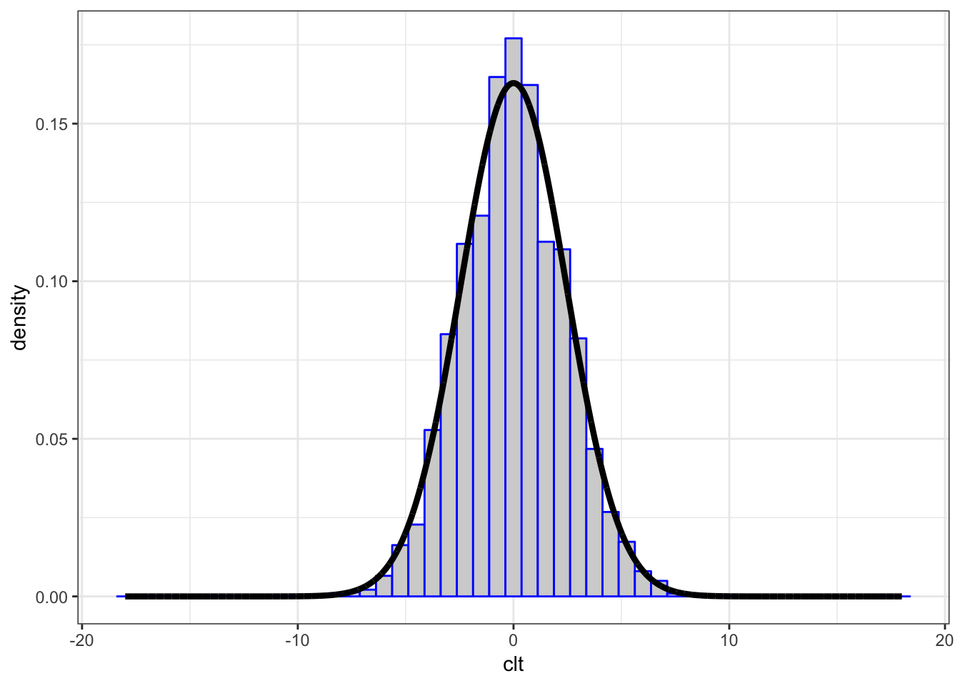
18.7 Example: Calculations
Let \(X_1, X_2, \ldots, X_{40}\) be iid Poisson(\(\lambda\)) with \(\lambda=6\).
We will form \(\sqrt{40}(\overline{X} - 6)\) over 10,000 realizations and compare their distribution to a Normal(0, 6) distribution.
> x <- replicate(n=1e4, expr=rpois(n=40, lambda=6),
+                simplify="matrix")
> x_bar <- apply(x, 2, mean)
> clt <- sqrt(40)*(x_bar - 6)
>
> df <- data.frame(clt=clt, x = seq(-18,18,length.out=1e4),
+                  y = dnorm(seq(-18,18,length.out=1e4),
+                            sd=sqrt(6)))
18.8 Example: Plot
> ggplot(data=df) +
+   geom_histogram(aes(x=clt, y=..density..), color="blue",
+                  fill="lightgray", binwidth=0.75) +
+   geom_line(aes(x=x, y=y), size=1.5)