52 Goodness of Fit

52.1 Rationale

Sometimes we want to figure out which probability distribution is a reasonable model for the data.

This is related to nonparametric inference in that we wish to go from being in a nonparametric framework to a parametric framework.

Goodness of fit (GoF) tests allow one to perform a hypothesis test of how well a particular parametric probability model explains variation observed in a data set.

52.2 Chi-Square GoF Test

Suppose we have data generating process \(X_1, X_2, \ldots, X_n {\; \stackrel{\text{iid}}{\sim}\;}F\) for some probability distribution \(F\). We wish to test \(H_0: F \in \{F_{{\boldsymbol{\theta}}}: {\boldsymbol{\theta}}\in \boldsymbol{\Theta} \}\) vs \(H_1: \mbox{not } H_0\). Suppose that \(\boldsymbol{\Theta}\) is \(d\)-dimensional.

Divide the support of \(\{F_{{\boldsymbol{\theta}}}: {\boldsymbol{\theta}}\in \boldsymbol{\Theta} \}\) into \(k\) bins \(I_1, I_2, \ldots, I_k\).

For \(j=1, 2, \ldots, k\), calculate

\[ q_j({\boldsymbol{\theta}}) = \int_{I_j} dF_{{\boldsymbol{\theta}}}(x). \]

Suppose we observe data \(x_1, x_2, \ldots, x_n\). For \(j = 1, 2, \ldots, k\), let \(n_j\) be the number of values \(x_i \in I_j\).

Let \(\tilde{\theta}_1, \tilde{\theta}_2, \ldots, \tilde{\theta}_d\) be the values that maximize the multinomial likelihood

\[ \prod_{j=1}^k q_j({\boldsymbol{\theta}})^{n_j}. \]

Form GoF statistic

\[ s({\boldsymbol{x}}) = \sum_{j=1}^k \frac{\left(n_j - n q_j\left(\tilde{{\boldsymbol{\theta}}} \right) \right)^2}{n q_j\left(\tilde{{\boldsymbol{\theta}}} \right)} \]

When \(H_0\) is true, \(S \sim \chi^2_v\) where \(v = k - d - 1\). The p-value is calculated by \(\Pr(S^* \geq s({\boldsymbol{x}}))\) where \(S^* \sim \chi^2_{k-d-1}\).

52.3 Example: Hardy-Weinberg

Suppose at your favorite SNP, we observe genotypes from 100 randomly sampled individuals as follows:

AA	AT	TT
28	60	12

If we code these genotypes as 0, 1, 2, testing for Hardy-Weinberg equilibrium is equivalent to testing whether \(X_1, X_2, \ldots, X_{100} {\; \stackrel{\text{iid}}{\sim}\;}\mbox{Binomial}(2, \theta)\) for some unknown allele frequency of T, \(\theta\).

The parameter dimension is such that \(d=1\). We will also set \(k=3\), where each bin is a genotype. Therefore, we have \(n_1 = 28\), \(n_2 = 60\), and \(n_3 = 12\). Also,

\[ q_1(\theta) = (1-\theta)^2, \ \ q_2(\theta) = 2 \theta (1-\theta), \ \ q_3(\theta) = \theta^2. \]

 

Forming the multinomial likelihood under these bin probabilities, we find \(\tilde{\theta} = (n_2 + 2n_3)/(2n)\). The degrees of freedom of the \(\chi^2_v\) null distribution is \(v = k - d - 1 = 3 - 1 - 1 = 1\).

Let’s carry out the test in R.

> n <- 100
> nj <- c(28, 60, 12)
> 
> # parameter estimates
> theta <- (nj[2] + 2*nj[3])/(2*n)
> qj <- c((1-theta)^2, 2*theta*(1-theta), theta^2)
> 
> # gof statistic
> s <- sum((nj - n*qj)^2 / (n*qj))
> 
> # p-value
> 1-pchisq(s, df=1)
[1] 0.02059811

52.4 Kolmogorov–Smirnov Test

The KS test can be used to compare a sample of data to a particular distribution, or to compare two samples of data. The former is a parametric GoF test, and the latter is a nonparametric test of equal distributions.

52.5 One Sample KS Test

Suppose we have data generating process \(X_1, X_2, \ldots, X_n \sim F\) for some probability distribution \(F\). We wish to test \(H_0: F = F_{{\boldsymbol{\theta}}}\) vs \(H_1: F \not= F_{{\boldsymbol{\theta}}}\) for some parametric distribution \(F_{{\boldsymbol{\theta}}}\).

For observed data \(x_1, x_2, \ldots, x_n\) we form the edf \(\hat{F}_{{\boldsymbol{x}}}\) and test-statistic

\[ D({\boldsymbol{x}}) = \sup_{z} \left| \hat{F}_{{\boldsymbol{x}}}(z) - F_{{\boldsymbol{\theta}}}(z) \right|. \]

The null distribution of this test can be approximated based on a stochastic process called the Brownian bridge.

52.6 Two Sample KS Test

Suppose \(X_1, X_2, \ldots, X_m {\; \stackrel{\text{iid}}{\sim}\;}F_X\) and \(Y_1, Y_2, \ldots, Y_n {\; \stackrel{\text{iid}}{\sim}\;}F_Y\). We wish to test \(H_0: F_X = F_Y\) vs \(H_1: F_X \not= F_Y\).

For observed data \(x_1, x_2, \ldots, x_m\) and \(y_1, y_2, \ldots, y_n\) we form the edf’s \(\hat{F}_{{\boldsymbol{x}}}\) and \(\hat{F}_{\boldsymbol{y}}\). We then form test-statistic

\[ D({\boldsymbol{x}},\boldsymbol{y}) = \sup_{z} \left| \hat{F}_{{\boldsymbol{x}}}(z) - \hat{F}_{\boldsymbol{y}}(z) \right|. \]

The null distribution of this statistic can be approximated using results on edf’s.

Both of these tests can be carried out using the ks.test() function in R.

ks.test(x, y, ...,
        alternative = c("two.sided", "less", "greater"),
        exact = NULL)

52.7 Example: Exponential vs Normal

Two sample KS test.

> x <- rnorm(100, mean=1)
> y <- rexp(100, rate=1)
> wilcox.test(x, y)

    Wilcoxon rank sum test with continuity correction

data:  x and y
W = 5021, p-value = 0.9601
alternative hypothesis: true location shift is not equal to 0
> ks.test(x, y)

    Two-sample Kolmogorov-Smirnov test

data:  x and y
D = 0.19, p-value = 0.0541
alternative hypothesis: two-sided

> qqplot(x, y); abline(0,1)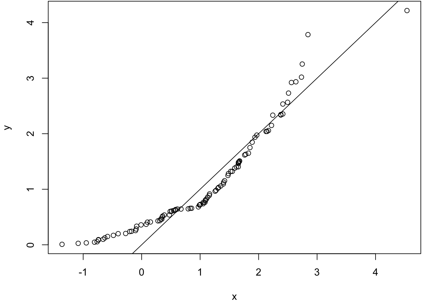

One sample KS tests.

> ks.test(x=x, y="pnorm")

    One-sample Kolmogorov-Smirnov test

data:  x
D = 0.41398, p-value = 2.554e-15
alternative hypothesis: two-sided
> 
> ks.test(x=x, y="pnorm", mean=1)

    One-sample Kolmogorov-Smirnov test

data:  x
D = 0.068035, p-value = 0.7436
alternative hypothesis: two-sided

Standardize (mean center, sd scale) the observations before comparing to a Normal(0,1) distribution.

> ks.test(x=((x-mean(x))/sd(x)), y="pnorm")

    One-sample Kolmogorov-Smirnov test

data:  ((x - mean(x))/sd(x))
D = 0.05896, p-value = 0.8778
alternative hypothesis: two-sided
> 
> ks.test(x=((y-mean(y))/sd(y)), y="pnorm")

    One-sample Kolmogorov-Smirnov test

data:  ((y - mean(y))/sd(y))
D = 0.14439, p-value = 0.03092
alternative hypothesis: two-sided