46 MCMC Example
46.1 Single Nucleotide Polymorphisms
SNPs
46.3 Gibbs Sampling Approach
The Bayesian Gibbs sampling approach to inferring the PSD model touches on many important ideas, such as conjugate priors and mixture models.
We will focus on a version of this model for diploid SNPs.
46.4 The Data
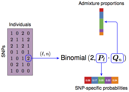
\(\boldsymbol{X}\), a \(L \times N\) matrix consisting of the genotypes, coded as \(0,1,2\). Each row is a SNP, each column is an individual.
In order for this model to work, the data needs to be broken down into “phased” genotypes. For the 0 and 2 cases, it’s obvious how to do this, and for the 1 case, it’ll suffice for this model to randomly assign the alleles to chromosomes. We will explore phasing more on HW4.
Thus, we wind up with two {0, 1} binary matrices \(\boldsymbol{X}_A\) and \(\boldsymbol{X}_B\), both \(L \times N\). We will refer to allele \(A\) and allele \(B\). Note \({\boldsymbol{X}}= {\boldsymbol{X}}_A + {\boldsymbol{X}}_B\).
46.5 Model Components
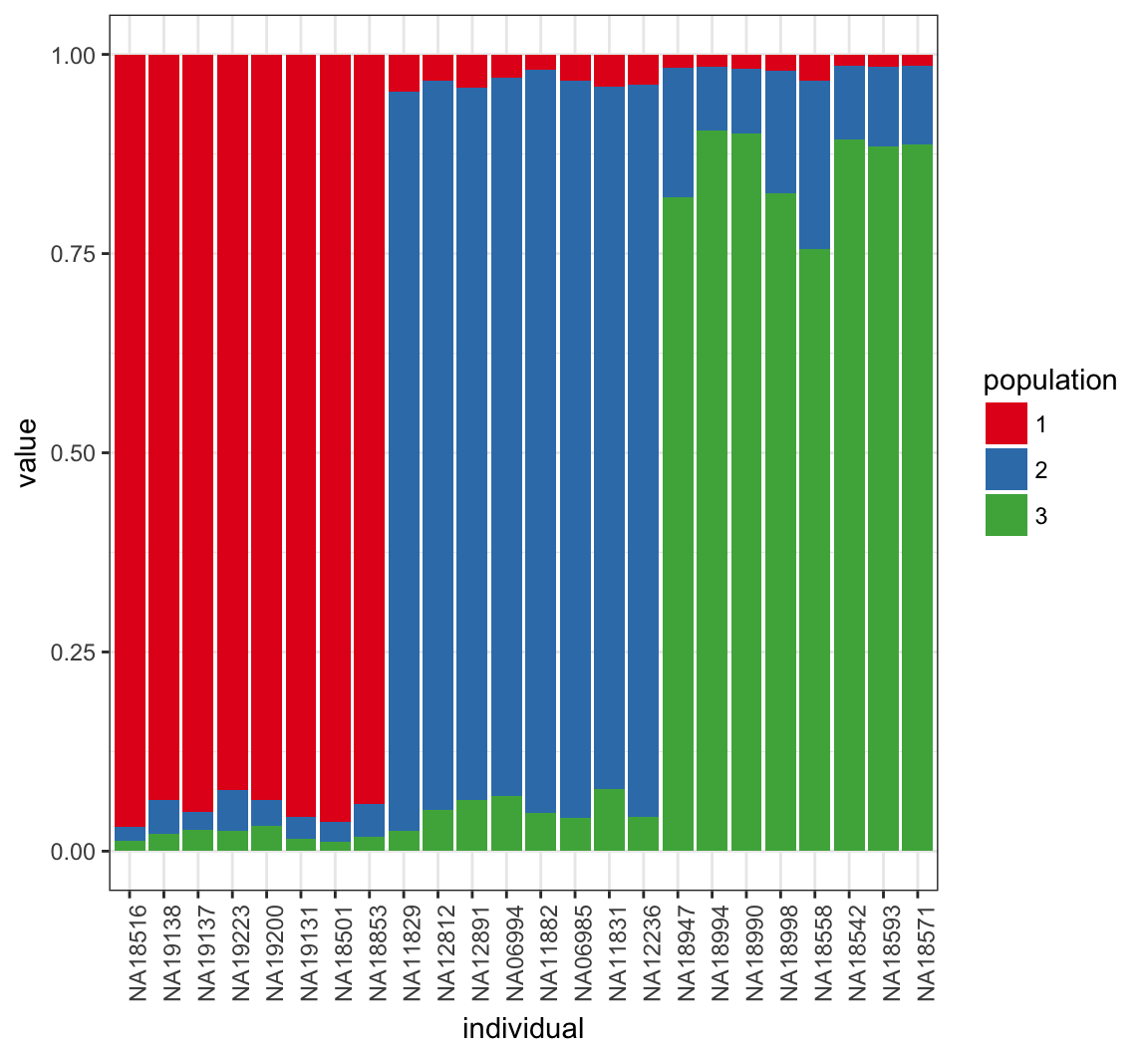
- \(K\), the number of populations that we model the genotypes as admixtures of. This is chosen before inference.
- \(\boldsymbol{Q}\), a \(N \times K\) matrix, the admixture proportions, values are in the interval \([0, 1]\) and rows are constrained to sum to 1.
- \(\boldsymbol{P}\), a \(L \times K\) matrix, the allele frequencies for each population, values are in the interval \([0, 1]\).
- \(\boldsymbol{Z}_A\) and \(\boldsymbol{Z}_B\), two \(L \times N\) matrices that tell us which population the respective allele is from. Elements consist of the integers between \(1\) and \(K\). This is a hidden variable.
46.6 The Model
- Each allele (elements of \(\boldsymbol{X}_A\) and \(\boldsymbol{X}_B\)) is a Bernoulli random variable, with success probability determined by which population that allele is assigned to (i.e., depends on \(\boldsymbol{Z}_A\), \(\boldsymbol{Z}_B\), and \(\boldsymbol{P}\)).
- We put a uniform Beta prior, i.e., \(\operatorname{Beta}(1, 1)\), on each element of \(\boldsymbol{P}\).
- We put a uniform Dirichlet prior, i.e., \(\operatorname{Dirichlet(1,\ldots,1)}\), on each row of \(\boldsymbol{Q}\).
- \(\boldsymbol{Z}_A\) and \(\boldsymbol{Z}_B\) are \(K\)-class Multinomial draws where the probability of drawing each class is determined by each row of \(Q\).
46.7 Conditional Independence
The key observation is to understand which parts of the model are dependent on each other in the data generating process.
- The data \(\boldsymbol{X}_A\) and \(\boldsymbol{X}_B\) depends directly on \(\boldsymbol{Z}_A\), \(\boldsymbol{Z}_B\), and \(\boldsymbol{P}\) (not \(\boldsymbol{Q}\)!).
- The latent variable \(\boldsymbol{Z}_A\) and \(\boldsymbol{Z}_B\) depend only on \(\boldsymbol{Q}\) and they’re conditionally independent given \(\boldsymbol{Q}\).
- \(\boldsymbol{Q}\) and \(\boldsymbol{P}\) depend only on their priors.
\(\Pr(\boldsymbol{X}_A, \boldsymbol{X}_B, \boldsymbol{Z}_A, \boldsymbol{Z}_B, \boldsymbol{P}, \boldsymbol{Q}) =\)
\(\Pr(\boldsymbol{X}_A, \boldsymbol{X}_B | \boldsymbol{Z}_A, \boldsymbol{Z}_B, \boldsymbol{P}) \Pr(\boldsymbol{Z}_A | \boldsymbol{Q}) \Pr(\boldsymbol{Z}_B | \boldsymbol{Q}) \Pr(\boldsymbol{P}) \Pr(\boldsymbol{Q})\)
46.8 The Posterior
We desire to compute the posterior distribution \(\Pr(\boldsymbol{P}, \boldsymbol{Q}, \boldsymbol{Z}_A, \boldsymbol{Z}_B | \boldsymbol{X}_A, \boldsymbol{X}_B)\). Gibbs sampling tells us if we can construct conditional distributions for each random variable in our model, then iteratively sampling and updating our model parameters will result in a stationary distribution that is the same as the posterior distribution.
Gibbs sampling is an extremely powerful approach for this model because we can utilize conjugate priors as well as the independence of various parameters in the model to compute these conditional distributions.
46.9 Full Conditional for \(\boldsymbol{Q}\)
Note that \(\boldsymbol{Z}_A\) and \(\boldsymbol{Z}_B\) are the only parts of this model that directly depend on \(\boldsymbol{Q}\).
\[\begin{align*} &\Pr(Q_n | \boldsymbol{Q}_{-n}, \boldsymbol{Z}_A, \boldsymbol{Z}_B, \boldsymbol{P}, \boldsymbol{X}_A, \boldsymbol{X}_B)\\ =& \Pr(Q_n | \boldsymbol{Z}_A, \boldsymbol{Z}_B) \\ \propto& \Pr(Z_{An}, Z_{Bn} | Q_n) \Pr(Q_n)\\ =& \Pr(Z_{An} | Q_n) \Pr(Z_{Bn} | Q_n) \Pr(Q_n)\\ \propto& \left( \prod_{\ell=1}^L \prod_{k=1}^K Q_{nk}^{\mathbb{1}(Z_{An\ell}=k)+\mathbb{1}(Z_{Bn\ell}=k)} \right) \end{align*}\]\[=\prod_{k=1}^K Q_{nk}^{S_{nk}}\]
where \(S_{nk}\) is simply the count of the number of alleles for individual \(n\) that got assigned to population \(k\).
Thus, \(Q_n | \boldsymbol{Z}_A, \boldsymbol{Z}_B \sim \operatorname{Dirichlet}(S_{j1}+1, \ldots, S_{jk}+1)\),.
We could have guessed that this distribution is Dirichlet given that \(\boldsymbol{Z}_A\) and \(\boldsymbol{Z}_B\) are multinomial! Let’s use conjugacy to help us in the future.
46.10 Full Conditional for \(\boldsymbol{P}\)
\[\begin{align*} &\Pr(P_\ell | \boldsymbol{P}_{-\ell}, \boldsymbol{Z}_A, \boldsymbol{Z}_B, \boldsymbol{Q}, \boldsymbol{X}_A, \boldsymbol{X}_B) \\ \propto& \Pr(\boldsymbol{X}_{A\ell}, \boldsymbol{X}_{B\ell} | P_\ell, \boldsymbol{Z}_{A\ell}, \boldsymbol{Z}_{B\ell}) \Pr(P_\ell) \end{align*}\]We know \(\Pr(\boldsymbol{X}_{A\ell}, \boldsymbol{X}_{B\ell} | P_\ell, \boldsymbol{Z}_{A\ell}, \boldsymbol{Z}_{B\ell})\) will be Bernoulli and \(\Pr(P_\ell)\) will be beta, so the full conditional will be beta as well. In fact, the prior is uniform so it vanishes from the RHS.
Thus, all we have to worry about is the Bernoulli portion \(\Pr(\boldsymbol{X}_{A\ell}, \boldsymbol{X}_{B\ell} | P_\ell, \boldsymbol{Z}_{A\ell}, \boldsymbol{Z}_{B\ell})\). Here, we observe that if the \(\boldsymbol{Z}_A\) and \(\boldsymbol{Z}_B\) are “known”, then we known which value of \(P_\ell\) to plug into our Bernoulli for \(\boldsymbol{X}_A\) and \(\boldsymbol{X}_B\). Following the Week 6 lectures, we find that the full conditional for \(\boldsymbol{P}\) is:
\[P_{\ell k} | \boldsymbol{Z}_A, \boldsymbol{Z}_B, \boldsymbol{X}_A, \boldsymbol{X}_B \sim \operatorname{Beta}(1+T_{\ell k 0}, 1+T_{\ell k 1})\]
where \(T_{\ell k 0}\) is the total number of 0 alleles at SNP \(\ell\) for population \(k\), and \(T_{\ell k 1}\) is the analogous quantity for the 1 allele.
46.11 Full Conditional \(\boldsymbol{Z}_A\) & \(\boldsymbol{Z}_B\)
We’ll save some math by first noting that alleles \(A\) and \(B\) are independent of each other, so we can write this for only \(\boldsymbol{Z}_A\) without losing any information. Also, all elements of \(\boldsymbol{Z}_A\) are independent of each other. Further, note that each element of \(\boldsymbol{Z}_A\) is a single multinomial draw, so we are working with a discrete random variable.
\[\begin{align*} &\Pr(Z_{A\ell n}=k | \boldsymbol{X}_A, \boldsymbol{Q}, \boldsymbol{P}) \\ =& \Pr (Z_{A\ell n}=k | X_{A \ell n}, Q_n, P_\ell) \\ \propto & \Pr(X_{A \ell n} | Z_{A\ell n}=k, Q_n, P_\ell) \Pr(Z_{A\ell n}=k | Q_n, P_\ell) \end{align*}\]We can look at the two factors. First:
\[\Pr(Z_{A\ell n}=k | Q_n, P_\ell) = \Pr(Z_{A\ell n}=k | Q_n) = Q_{nk}\]
Then:
\[\Pr(X_{A \ell n} | Z_{A\ell n}=k, Q_n, P_\ell) = P_{\ell k}\]
Thus, we arrive at the formula:
\[\Pr(Z_{A\ell n}=k | \boldsymbol{X}_A, \boldsymbol{Q}, \boldsymbol{P}) \propto P_{\ell k} Q_{n k}\]
46.12 Gibbs Sampling Updates
It’s neat that we wind up just iteratively counting the various discrete random variables along different dimensions.
\[\begin{align*} Q_n | \boldsymbol{Z}_A, \boldsymbol{Z}_B &\sim \operatorname{Dirichlet}(S_{j1}+1, \ldots, S_{jk}+1)\\ P_{\ell k} | \boldsymbol{Z}_A, \boldsymbol{Z}_B, \boldsymbol{X}_A, \boldsymbol{X}_B &\sim \operatorname{Beta}(1+T_{\ell k 0}, 1+T_{\ell k 1}) \\ Z_{A\ell n} | \boldsymbol{X}_A, \boldsymbol{Q}, \boldsymbol{P} &\sim \operatorname{Multinomial}\left(\frac{P_\ell * Q_n}{P_\ell \cdot Q_n}\right) \end{align*}\]where \(*\) means element-wise vector multiplication.
46.13 Implementation
The Markov chain property means that we can’t use vectorization forward in time, so R is not the best way to implement this algorithm.
That being said, we can vectorize the pieces that we can and demonstrate what happens.
46.14 Matrix-wise rdirichlet Function
Drawing from a Dirichlet is easy and vectorizable because it consists of normalizing independent gamma draws.
> rdirichlet <- function(alpha) {
+   m <- nrow(alpha)
+   n <- ncol(alpha)
+   x <- matrix(rgamma(m * n, alpha), ncol = n)
+   x/rowSums(x)
+ }
46.15 Inspect Data
> dim(Xa)
[1] 400  24
> X[1:3,1:3]
           NA18516 NA19138 NA19137
rs2051075        0       1       2
rs765546         2       2       0
rs10019399       2       2       2
> Xa[1:3,1:3]
           NA18516 NA19138 NA19137
rs2051075        0       0       1
rs765546         1       1       0
rs10019399       1       1       1
46.16 Model Parameters
> L <- nrow(Xa)
> N <- ncol(Xa)
>
> K <- 3
>
> Za <- matrix(sample(1:K, L*N, replace=TRUE), L, N)
> Zb <- matrix(sample(1:K, L*N, replace=TRUE), L, N)
> P <- matrix(0, L, K)
> Q <- matrix(0, N, K)
46.17 Update \(\boldsymbol{P}\)
> update_P <- function() {
+   Na_0 <- Za * (Xa==0)
+   Na_1 <- Za * (Xa==1)
+   Nb_0 <- Zb * (Xb==0)
+   Nb_1 <- Zb * (Xb==1)
+   for(k in 1:K) {
+     N0 <- rowSums(Na_0==k)+rowSums(Nb_0==k)
+     N1 <- rowSums(Na_1==k)+rowSums(Nb_1==k)
+     P[,k] <- rdirichlet(1+cbind(N1, N0))[,1]
+   }
+   P
+ }
46.18 Update \(\boldsymbol{Q}\)
> update_Q <- function() {
+   M_POP0 <- apply(Za, 2, function(x) {tabulate(x, nbins=K)} )
+   M_POP1 <- apply(Zb, 2, function(x) {tabulate(x, nbins=K)} )
+
+   rdirichlet(t(1+M_POP0+M_POP1))
+ }
46.19 Update (Each) \(\boldsymbol{Z}\)
> update_Z <- function(X) {
+   Z <- matrix(0, nrow(X), ncol(X))
+   for(n in 1:N) {
+     PZ0 <- t(t((1-P)) * Q[n,])
+     PZ1 <- t(t(P) * Q[n,])
+     PZ <- X[,n]*PZ1 + (1-X[,n])*PZ0
+     Z[,n] <- apply(PZ, 1, function(p){sample(1:K, 1, prob=p)})
+   }
+   Z
+ }
46.20 Model Log-likelihood Function
> model_ll <- function() {
+   AFa <- t(sapply(1:L, function(i){P[i,][Za[i,]]}))
+   AFb <- t(sapply(1:L, function(i){P[i,][Zb[i,]]}))
+   # hint, hint, HW3
+   sum(dbinom(Xa, 1, AFa, log=TRUE)) +
+     sum(dbinom(Xb, 1, AFb, log=TRUE))
+ }
46.21 MCMC Configuration
> MAX_IT <- 20000
> BURNIN <- 5000
> THIN <- 20
>
> QSUM <- matrix(0, N, K)
>
> START <- 200
> TAIL <- 500
> LL_start <- rep(0, START)
> LL_end <- rep(0, TAIL)
46.22 Run Sampler
> set.seed(1234)
>
> for(it in 1:MAX_IT) {
+   P <- update_P()
+   Q <- update_Q()
+   Za <- update_Z(Xa)
+   Zb <- update_Z(Xb)
+
+   if(it > BURNIN && it %% THIN == 0) {QSUM <- QSUM+Q}
+   if(it <= START) {LL_start[it] <- model_ll()}
+   if(it > MAX_IT-TAIL) {LL_end[it-(MAX_IT-TAIL)] <- model_ll()}
+ }
>
> Q_MEAN <- QSUM/((MAX_IT-BURNIN)/THIN)
46.23 Posterior Mean of \(\boldsymbol{Q}\)
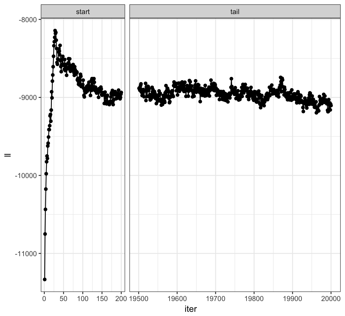
46.24 Plot Log-likelihood Steps
Note both the needed burn-in and thinning.
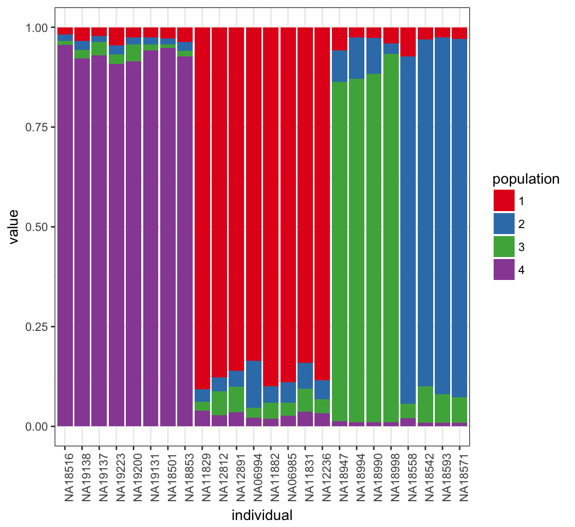
46.25 What Happens for K=4?
> K <- 4
> Za <- matrix(sample(1:K, L*N, replace=TRUE), L, N)
> Zb <- matrix(sample(1:K, L*N, replace=TRUE), L, N)
> P <- matrix(0, L, K)
> Q <- matrix(0, N, K)
> QSUM <- matrix(0, N, K)
46.26 Run Sampler Again
> for(it in 1:MAX_IT) {
+   P <- update_P()
+   Q <- update_Q()
+   Za <- update_Z(Xa)
+   Zb <- update_Z(Xb)
+
+   if(it > BURNIN && it %% THIN == 0) {
+     QSUM <- QSUM+Q
+   }
+ }
>
> Q_MEAN <- QSUM/((MAX_IT-BURNIN)/THIN)
46.27 Posterior Mean of \(\boldsymbol{Q}\)