60 OLS in R
R implements OLS of multiple explanatory variables exactly the same as with a single explanatory variable, except we need to show the sum of all explanatory variables that we want to use.
> lm(weight ~ height + sex, data=htwt)

Call:
lm(formula = weight ~ height + sex, data = htwt)

Coefficients:
(Intercept)       height         sexM
   -76.6167       0.8106       8.2269
60.1 Weight Regressed on Height + Sex
> summary(lm(weight ~ height + sex, data=htwt))

Call:
lm(formula = weight ~ height + sex, data = htwt)

Residuals:
    Min      1Q  Median      3Q     Max
-20.131  -4.884  -0.640   5.160  41.490

Coefficients:
            Estimate Std. Error t value Pr(>|t|)
(Intercept) -76.6167    15.7150  -4.875 2.23e-06 ***
height        0.8105     0.0953   8.506 4.50e-15 ***
sexM          8.2269     1.7105   4.810 3.00e-06 ***
---
Signif. codes:  0 '***' 0.001 '**' 0.01 '*' 0.05 '.' 0.1 ' ' 1

Residual standard error: 8.066 on 197 degrees of freedom
Multiple R-squared:  0.6372,    Adjusted R-squared:  0.6335
F-statistic:   173 on 2 and 197 DF,  p-value: < 2.2e-16
60.2 One Variable, Two Scales
We can include a single variable but on two different scales:
> htwt <- htwt %>% mutate(height2 = height^2)
> summary(lm(weight ~ height + height2, data=htwt))

Call:
lm(formula = weight ~ height + height2, data = htwt)

Residuals:
    Min      1Q  Median      3Q     Max
-24.265  -5.159  -0.499   4.549  42.965

Coefficients:
              Estimate Std. Error t value Pr(>|t|)
(Intercept) 107.117140 175.246872   0.611    0.542
height       -1.632719   2.045524  -0.798    0.426
height2       0.008111   0.005959   1.361    0.175

Residual standard error: 8.486 on 197 degrees of freedom
Multiple R-squared:  0.5983,    Adjusted R-squared:  0.5943
F-statistic: 146.7 on 2 and 197 DF,  p-value: < 2.2e-16
60.3 Interactions
It is possible to include products of explanatory variables, which is called an interaction.
> summary(lm(weight ~ height + sex + height:sex, data=htwt))

Call:
lm(formula = weight ~ height + sex + height:sex, data = htwt)

Residuals:
    Min      1Q  Median      3Q     Max
-20.869  -4.835  -0.897   4.429  41.122

Coefficients:
            Estimate Std. Error t value Pr(>|t|)
(Intercept) -45.6730    22.1342  -2.063   0.0404 *
height        0.6227     0.1343   4.637 6.46e-06 ***
sexM        -55.6571    32.4597  -1.715   0.0880 .
height:sexM   0.3729     0.1892   1.971   0.0502 .
---
Signif. codes:  0 '***' 0.001 '**' 0.01 '*' 0.05 '.' 0.1 ' ' 1

Residual standard error: 8.007 on 196 degrees of freedom
Multiple R-squared:  0.6442,    Adjusted R-squared:  0.6388
F-statistic: 118.3 on 3 and 196 DF,  p-value: < 2.2e-16
60.4 More on Interactions
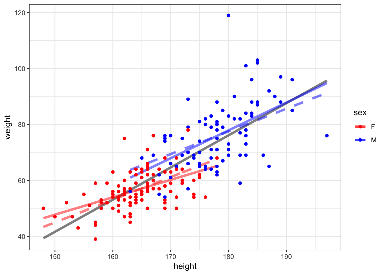
What happens when there is an interaction between a quantitative explanatory variable and a factor explanatory variable? In the next plot, we show three models:
- Grey solid:
lm(weight ~ height, data=htwt) - Color dashed:
lm(weight ~ height + sex, data=htwt) - Color solid:
lm(weight ~ height + sex + height:sex, data=htwt)
60.5 Visualizing Three Different Models