42 EM Examples

42.1 Normal Mixture Model

Returning to the Normal mixture model introduced earlier, we first calculate

\[ \log f({\boldsymbol{x}}, {\boldsymbol{z}}; {\boldsymbol{\theta}}) = \sum_{i=1}^n \sum_{k=1}^K z_{ik} \log \pi_k + z_{ik} \log \phi(x_i; \mu_k, \sigma^2_k) \]

where

\[ \phi(x_i; \mu_k, \sigma^2_k) = \frac{1}{\sqrt{2\pi\sigma^2_k}} \exp \left\{ -\frac{(x_i - \mu_k)^2}{2 \sigma^2_k} \right\}. \]

In caculating

\[Q({\boldsymbol{\theta}}, {\boldsymbol{\theta}}^{(t)}) = {\operatorname{E}}_{{\boldsymbol{Z}}|{\boldsymbol{X}}={\boldsymbol{x}}}\left[\log f({\boldsymbol{x}}, {\boldsymbol{Z}}; {\boldsymbol{\theta}}); {\boldsymbol{\theta}}^{(t)}\right]\]

we only need to know \({\operatorname{E}}_{{\boldsymbol{Z}}|{\boldsymbol{X}}={\boldsymbol{x}}}[Z_{ik} | {\boldsymbol{x}}; {\boldsymbol{\theta}}]\), which turns out to be

\[ {\operatorname{E}}_{{\boldsymbol{Z}}|{\boldsymbol{X}}={\boldsymbol{x}}}[Z_{ik} | {\boldsymbol{x}}; {\boldsymbol{\theta}}] = \frac{\pi_k \phi(x_i; \mu_k, \sigma^2_k)}{\sum_{j=1}^K \pi_j \phi(x_i; \mu_j, \sigma^2_j)}. \]

Note that we take

\[Q({\boldsymbol{\theta}}, {\boldsymbol{\theta}}^{(t)}) = {\operatorname{E}}_{{\boldsymbol{Z}}|{\boldsymbol{X}}={\boldsymbol{x}}}\left[\log f({\boldsymbol{x}}, {\boldsymbol{Z}}; {\boldsymbol{\theta}}); {\boldsymbol{\theta}}^{(t)}\right]\]

so the parameter in \(\log f({\boldsymbol{x}}, {\boldsymbol{Z}}; {\boldsymbol{\theta}})\) is a free \({\boldsymbol{\theta}}\), but the paramaters used to take the conditional expectation of \({\boldsymbol{Z}}\) are fixed at \({\boldsymbol{\theta}}^{(t)}\). Let’s define

\[ \hat{z}_{ik}^{(t)} = {\operatorname{E}}\left[z_{ik} | {\boldsymbol{x}}; {\boldsymbol{\theta}}^{(t)}\right] = \frac{\pi^{(t)}_k \phi(x_i; \mu^{(t)}_k, \sigma^{2, (t)}_k)}{\sum_{j=1}^K \pi^{(t)}_j \phi(x_i; \mu^{(t)}_j, \sigma^{2, (t)}_j)}. \]

42.2 E-Step

We calculate

\[Q({\boldsymbol{\theta}}, {\boldsymbol{\theta}}^{(t)}) = {\operatorname{E}}_{{\boldsymbol{Z}}|{\boldsymbol{X}}={\boldsymbol{x}}}\left[\log f({\boldsymbol{x}}, {\boldsymbol{Z}}; {\boldsymbol{\theta}}); {\boldsymbol{\theta}}^{(t)}\right]\] \[ = \sum_{i=1}^n \sum_{k=1}^K \hat{z}_{ik}^{(t)} \log \pi_k + \hat{z}_{ik}^{(t)} \log \phi(x_i; \mu_k, \sigma^2_k)\]

At this point the parameters making up \(\hat{z}_{ik}^{(t)}\) are fixed at \({\boldsymbol{\theta}}^{(t)}\).

42.3 M-Step

We now caculate \({\boldsymbol{\theta}}^{(t+1)} = {\text{argmax}}_{{\boldsymbol{\theta}}} Q({\boldsymbol{\theta}}, {\boldsymbol{\theta}}^{(t)}\), which yields:

\[ \pi_k^{(t+1)} = \frac{\sum_{i=1}^n \hat{z}_{ik}^{(t)}}{n} \]

\[ \mu_k^{(t+1)} = \frac{\sum_{i=1}^n \hat{z}_{ik}^{(t)} x_i}{\sum_{i=1}^n \hat{z}_{ik}^{(t)}} \]

\[ \sigma_k^{2, (t+1)} = \frac{\sum_{i=1}^n \hat{z}_{ik}^{(t)} \left(x_i - \mu_k^{(t+1)} \right)^2}{\sum_{i=1}^n \hat{z}_{ik}^{(t)}} \]

Note: You need to use a Lagrange multiplier to obtain \(\{\pi_k^{(t+1)}\}_{k=1}^{K}\).

42.4 Caveat

If we assign one and only one data point to mixture component \(k\), meaning \(\mu_k^{(t)} = x_i\) and \(\hat{z}_{ik}^{(t)}=1\) for some \(k\) and \(i\), then as \(\sigma^{2, (t)}_k \rightarrow 0\), the likelihood goes to \(\infty\).

Therefore, when implementing the EM algorithm for this particular Normal mixture model, we have to be careful to bound all \(\sigma^{2, (t)}_k\) away from zero and avoid this scenario.

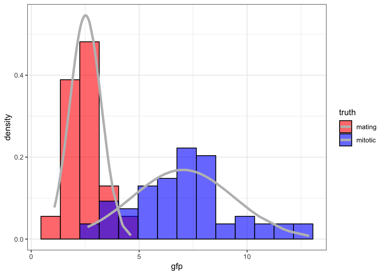
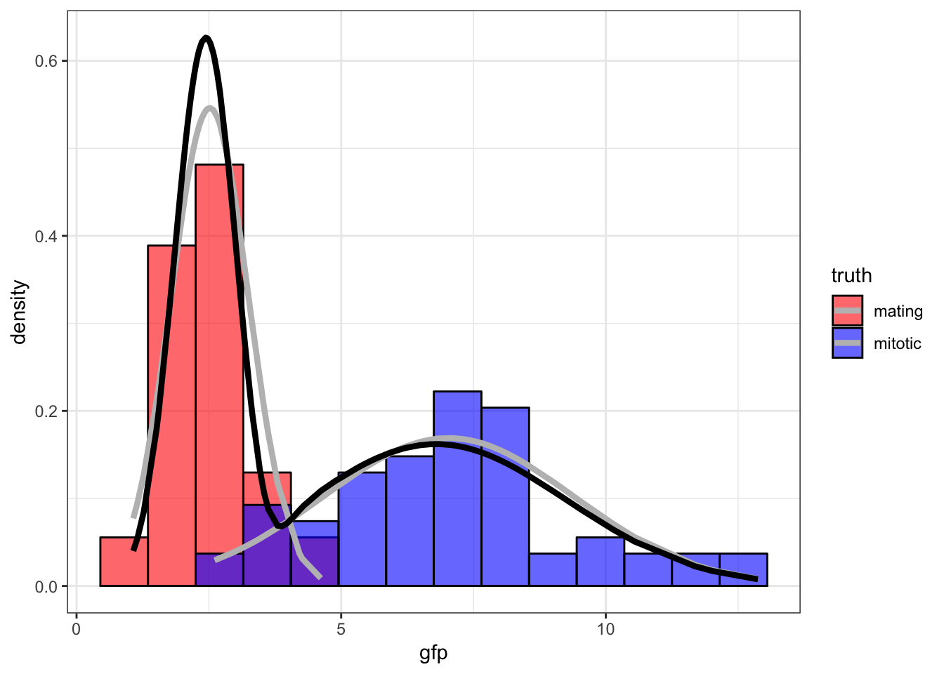
42.5 Yeast Gene Expression

Measured ratios of the nuclear to cytoplasmic fluorescence for a protein-GFP construct that is hypothesized as being nuclear in mitotic cells and largely cytoplasmic in mating cells.

42.6 Initialize Values

> set.seed(508)
> B <- 100
> p <- rep(0,B)
> mu1 <- rep(0,B)
> mu2 <- rep(0,B)
> s1 <- rep(0,B)
> s2 <- rep(0,B)
> p[1] <- runif(1, min=0.1, max=0.9)
> mu.start <- sample(x, size=2, replace=FALSE)
> mu1[1] <- min(mu.start)
> mu2[1] <- max(mu.start)
> s1[1] <- var(sort(x)[1:60])
> s2[1] <- var(sort(x)[61:120])
> z <- rep(0,120)

42.7 Run EM Algorithm

> for(i in 2:B) {
+   z <- (p[i-1]*dnorm(x, mean=mu2[i-1], sd=sqrt(s2[i-1])))/
+     (p[i-1]*dnorm(x, mean=mu2[i-1], sd=sqrt(s2[i-1])) + 
+        (1-p[i-1])*dnorm(x, mean=mu1[i-1], sd=sqrt(s1[i-1])))
+   mu1[i] <- sum((1-z)*x)/sum(1-z)
+   mu2[i] <- sum(z*x)/sum(z)
+   s1[i] <- sum((1-z)*(x-mu1[i])^2)/sum(1-z)
+   s2[i] <- sum(z*(x-mu2[i])^2)/sum(z)
+   p[i] <- sum(z)/length(z)
+ }
> 
> tail(cbind(mu1, s1, mu2, s2, p), n=3)
            mu1        s1    mu2       s2         p
 [98,] 2.455325 0.3637967 6.7952 6.058291 0.5340015
 [99,] 2.455325 0.3637967 6.7952 6.058291 0.5340015
[100,] 2.455325 0.3637967 6.7952 6.058291 0.5340015

42.8 Fitted Mixture Distribution

42.9 Bernoulli Mixture Model

As an exercise, derive the EM algorithm of the Bernoilli mixture model introduced earlier.

Hint: Replace \(\phi(x_i; \mu_k, \sigma^2_k)\) with the appropriate Bernoilli pmf.

42.10 Other Applications of EM

• Dealing with missing data
• Multiple imputation of missing data
• Truncated observations
• Bayesian hyperparameter estimation
• Hidden Markov models