55 Motivating Examples
55.1 Sample Correlation
Least squares regression “modelizes” correlation. Suppose we observe \(n\) pairs of data \((x_1, y_1), (x_2, y_2), \ldots, (x_n, y_n)\). Their sample correlation is
\[\begin{eqnarray} r_{xy} & = & \frac{\sum_{i=1}^n (x_i - \overline{x}) (y_i - \overline{y})}{\sqrt{\sum_{i=1}^n (x_i - \overline{x})^2 \sum_{i=1}^n (y_i - \overline{y})^2}} \\ \ & = & \frac{\sum_{i=1}^n (x_i - \overline{x}) (y_i - \overline{y})}{(n-1) s_x s_y} \end{eqnarray}\]where \(s_x\) and \(s_y\) are the sample standard deviations of each measured variable.
55.2 Example: Hand Size Vs. Height
> library("MASS")
> data("survey", package="MASS")
> head(survey)
     Sex Wr.Hnd NW.Hnd W.Hnd    Fold Pulse    Clap Exer Smoke Height
1 Female   18.5   18.0 Right  R on L    92    Left Some Never 173.00
2   Male   19.5   20.5  Left  R on L   104    Left None Regul 177.80
3   Male   18.0   13.3 Right  L on R    87 Neither None Occas     NA
4   Male   18.8   18.9 Right  R on L    NA Neither None Never 160.00
5   Male   20.0   20.0 Right Neither    35   Right Some Never 165.00
6 Female   18.0   17.7 Right  L on R    64   Right Some Never 172.72
       M.I    Age
1   Metric 18.250
2 Imperial 17.583
3     <NA> 16.917
4   Metric 20.333
5   Metric 23.667
6 Imperial 21.000
> ggplot(data = survey, mapping=aes(x=Wr.Hnd, y=Height)) +
+ geom_point() + geom_vline(xintercept=mean(survey$Wr.Hnd, na.rm=TRUE)) +
+ geom_hline(yintercept=mean(survey$Height, na.rm=TRUE))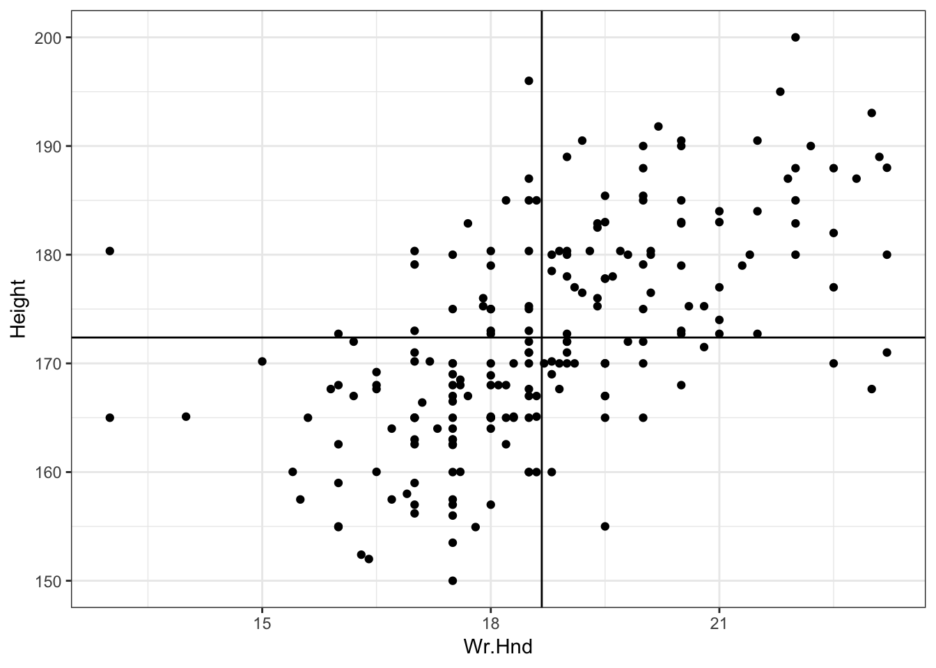
55.3 Cor. of Hand Size and Height
> cor.test(x=survey$Wr.Hnd, y=survey$Height)

    Pearson's product-moment correlation

data:  survey$Wr.Hnd and survey$Height
t = 10.792, df = 206, p-value < 2.2e-16
alternative hypothesis: true correlation is not equal to 0
95 percent confidence interval:
 0.5063486 0.6813271
sample estimates:
      cor
0.6009909
55.4 L/R Hand Sizes
> ggplot(data = survey) +
+   geom_point(aes(x=Wr.Hnd, y=NW.Hnd))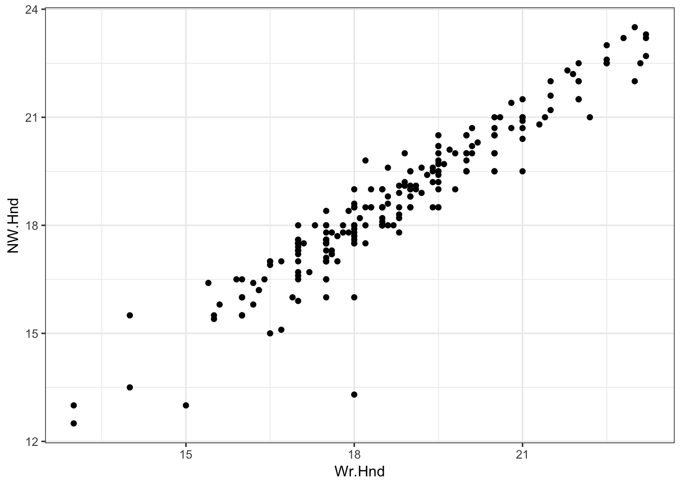
55.5 Correlation of Hand Sizes
> cor.test(x=survey$Wr.Hnd, y=survey$NW.Hnd)

    Pearson's product-moment correlation

data:  survey$Wr.Hnd and survey$NW.Hnd
t = 45.712, df = 234, p-value < 2.2e-16
alternative hypothesis: true correlation is not equal to 0
95 percent confidence interval:
 0.9336780 0.9597816
sample estimates:
      cor
0.9483103
55.6 Davis Data
> library("car")
> data("Davis", package="car")
Warning in data("Davis", package = "car"): data set 'Davis' not found
> htwt <- tbl_df(Davis)
> htwt[12,c(2,3)] <- htwt[12,c(3,2)]
> head(htwt)
# A tibble: 6 x 5
sex weight height repwt repht
<fct> <int> <int> <int> <int>
1 M 77 182 77 180
2 F 58 161 51 159
3 F 53 161 54 158
4 M 68 177 70 175
5 F 59 157 59 155
6 M 76 170 76 16555.7 Height and Weight
> ggplot(htwt) +
+   geom_point(aes(x=height, y=weight, color=sex), size=2, alpha=0.5) +
+   scale_color_manual(values=c("red", "blue"))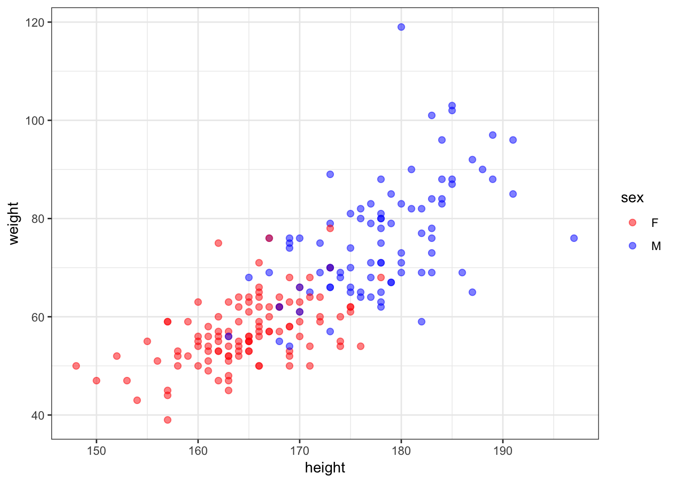
55.8 Correlation of Height and Weight
> cor.test(x=htwt$height, y=htwt$weight)

    Pearson's product-moment correlation

data:  htwt$height and htwt$weight
t = 17.04, df = 198, p-value < 2.2e-16
alternative hypothesis: true correlation is not equal to 0
95 percent confidence interval:
 0.7080838 0.8218898
sample estimates:
      cor
0.7710743
55.9 Correlation Among Females
> htwt %>% filter(sex=="F") %>%
+   cor.test(~ height + weight, data = .)

    Pearson's product-moment correlation

data:  height and weight
t = 6.2801, df = 110, p-value = 6.922e-09
alternative hypothesis: true correlation is not equal to 0
95 percent confidence interval:
 0.3627531 0.6384268
sample estimates:
      cor
0.5137293
55.10 Correlation Among Males
> htwt %>% filter(sex=="M") %>%
+   cor.test(~ height + weight, data = .)

    Pearson's product-moment correlation

data:  height and weight
t = 5.9388, df = 86, p-value = 5.922e-08
alternative hypothesis: true correlation is not equal to 0
95 percent confidence interval:
 0.3718488 0.6727460
sample estimates:
      cor
0.5392906
Why are the stratified correlations lower?