25 Hypothesis Tests
25.1 Example: HT on Fairness of a Coin
Suppose I claim that a specific coin is fair, i.e., that it lands on heads or tails with equal probability.
I flip it 20 times and it lands on heads 16 times.
- My data is \(x=16\) heads out of \(n=20\) flips.
- My data generation model is \(X \sim \mbox{Binomial}(20, p)\).
- I form the statistic \(\hat{p} = 16/20\) as an estimate of \(p\).
More formally, I want to test the hypothesis: \(H_0: p=0.5\) vs. \(H_1: p \not=0.5\) under the model \(X \sim \mbox{Binomial}(20, p)\) based on the test statistic \(\hat{p} = X/n\).
Let’s simulate 10,000 times what my estimate would look like if \(p=0.5\) and I repeated the 20 coin flips over and over.
> x <- replicate(n=1e4, expr=rbinom(1, size=20, prob=0.5))
> sim_p_hat <- x/20
> my_p_hat <- 16/20
The vector sim_p_hat contains 10,000 draws from the null distribution, i.e., the distribution of my test statstic \(\hat{p} = X/n\) when \(H_0: p=0.5\) is true.
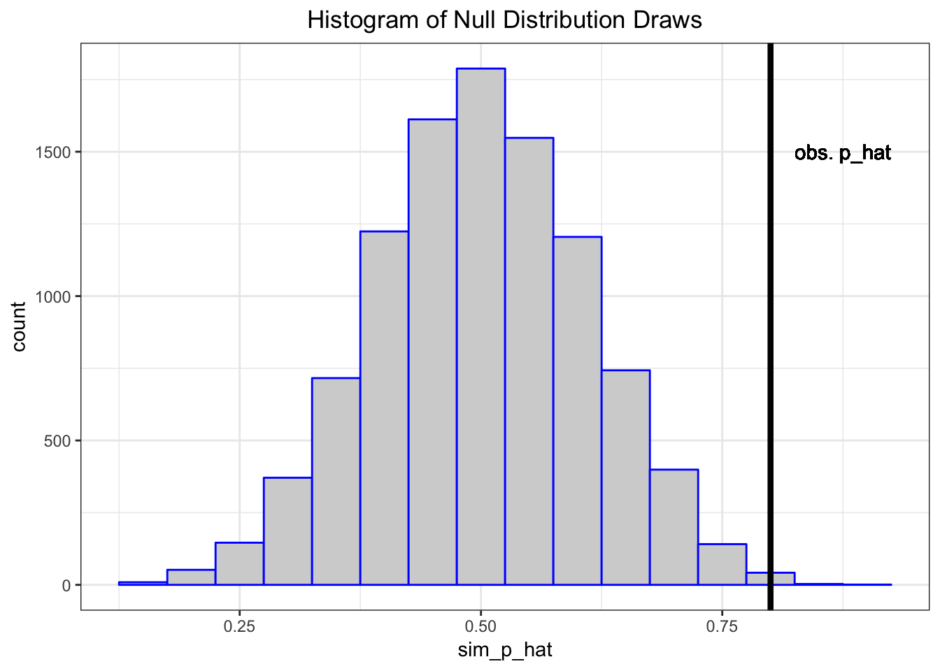
The deviation of the test statistic from the null hypothesis can be measured by \(|\hat{p} - 0.5|\).
Let’s compare our observed deviation \(|16/20 - 0.5|\) to the 10,000 simulated null data sets. Specifically, let’s calculate the frequency by which these 10,000 cases are as or more extreme than the observed test statistic.
> sum(abs(sim_p_hat-0.5) >= abs(my_p_hat-0.5))/1e4
[1] 0.0055
This quantity is called the p-value of the hypothesis test.
25.2 A Caveat
This example is a simplification of a more general framework for testing statistical hypotheses.
Given the intuition provided by the example, let’s now formalize these ideas.
25.3 Definition
- A hypothesis test or significance test is a formal procedure for comparing observed data with a hypothesis whose truth we want to assess
- The results of a test are expressed in terms of a probability that measures how well the data and the hypothesis agree
- The null hypothesis (\(H_0\)) is the statement being tested, typically the status quo
- The alternative hypothesis (\(H_1\)) is the complement of the null, and it is often the “interesting” state
25.4 Return to Normal Example
Let’s return to our Normal example in order to demonstrate the framework.
Suppose a simple random sample of \(n\) data points is collected so that the following model of the data is reasonable: \(X_1, X_2, \ldots, X_n\) are iid Normal(\(\mu\), \(\sigma^2\)).
The goal is to do test a hypothesis on \(\mu\), the population mean.
For simplicity, assume that \(\sigma^2\) is known (e.g., \(\sigma^2 = 1\)).
25.5 HTs on Parameter Values
Hypothesis tests are usually formulated in terms of values of parameters. For example:
\[H_0: \mu = 5\]
\[H_1: \mu \not= 5\]
Note that the choice of 5 here is arbitrary, for illustrative purposes only. In a typical real world problem, the values that define the hypotheses will be clear from the context.
25.6 Two-Sided vs. One-Sided HT
Hypothesis tests can be two-sided or one-sided:
\[H_0: \mu = 5 \mbox{ vs. } H_1: \mu \not= 5 \mbox{ (two-sided)}\]
\[H_0: \mu \leq 5 \mbox{ vs. } H_1: \mu > 5 \mbox{ (one-sided)}\]
\[H_0: \mu \geq 5 \mbox{ vs. } H_1: \mu < 5 \mbox{ (one-sided)}\]
25.7 Test Statistic
A test statistic is designed to quantify the evidence against the null hypothesis in favor of the alternative. They are usually defined (and justified using math theory) so that the larger the test statistic is, the more evidence there is.
For the Normal example and the two-sided hypothesis \((H_0: \mu = 5 \mbox{ vs. } H_1: \mu \not= 5)\), here is our test statistic:
\[ |z| = \frac{\left|\overline{x} - 5\right|}{\sigma/\sqrt{n}} \]
What would the test statistic be for the one-sided hypothesis tests?
25.8 Null Distribution (Two-Sided)
The null distribution is the sampling distribution of the test statistic when \(H_0\) is true.
We saw earlier that \(\frac{\overline{X} - \mu}{\sigma/\sqrt{n}} \sim \mbox{Normal}(0,1).\)
When \(H_0\) is true, then \(\mu=5\). So when \(H_0\) is true it follows that
\[Z = \frac{\overline{X} - 5}{\sigma/\sqrt{n}} \sim \mbox{Normal}(0,1)\]
and then probabiliy calculations on \(|Z|\) are straightforward. Note that \(Z\) is pivotal when \(H_0\) is true!
25.9 Null Distribution (One-Sided)
When performing a one-sided hypothesis test, such as \(H_0: \mu \leq 5 \mbox{ vs. } H_1: \mu > 5\), the null distribution is typically calculated under the “least favorable” value, which is the boundary value.
In this example it would be \(\mu=5\) and we would again utilize the null distribution \[Z = \frac{\overline{X} - 5}{\sigma/\sqrt{n}} \sim \mbox{Normal}(0,1).\]
25.10 P-values
The p-value is defined to be the probability that a test statistic from the null distribution is as or more extreme than the observed statistic. In our Normal example on the two-sided hypothesis test, the p-value is
\[{\rm Pr}(|Z^*| \geq |z|)\]
where \(Z^* \sim \mbox{Normal}(0,1)\) and \(|z|\) is the value of the test statistic calculated on the data (so it is a fixed number once we observe the data).
25.11 Calling a Test “Significant”
A hypothesis test is called statistically significant — meaning we reject \(H_0\) in favor of \(H_1\) — if its p-value is sufficiently small.
Commonly used cut-offs are 0.01 or 0.05, although these are not always appropriate and they are historical artifacts.
Applying a specific p-value cut-off to determine significance determines an error rate, which we define next.
25.12 Types of Errors
There are two types of errors that can be committed when performing a hypothesis test.
- A Type I error or false positive is when a hypothesis test is called signficant and the null hypothesis is actually true.
- A Type II error or false negative is when a hypothesis test is not called signficant and the alternative hypothesis is actually true.
25.13 Error Rates
- The Type I error rate or false positive rate is the probability of this type of error given that \(H_0\) is true.
- If a hypothesis test is called significant when p-value \(\leq \alpha\) then it has a Type I error rate equal to \(\alpha\).
- The Type II error rate or false negative rate is the probability of this type of error given that \(H_1\) is true.
- The power of a hypothesis test is \(1 -\) Type II error rate.
Hypothesis tests are usually derived with a goal to control the Type I error rate while maximizing the power.