75 Ridge Regression
75.1 Motivation
Ridge regression is a technique for shrinking the coefficients towards zero in linear models.
It also deals with collinearity among explanatory variables. Collinearity is the presence of strong correlation among two or more explanatory variables.
75.2 Optimization Goal
Under the OLS model assumptions, ridge regression fits model by minimizing the following:
\[ \sum_{j=1}^n \left(y_j - \sum_{i=1}^m \beta_{i} x_{ij}\right)^2 + \lambda \sum_{k=1}^m \beta_k^2. \]
Recall the \(\ell_2\) norm: \(\sum_{k=1}^m \beta_k^2 = \| {\boldsymbol{\beta}}\|^2_2\). Sometimes ridge regression is called \(\ell_2\) penalized regression.
As with natural cubic splines, the paramater \(\lambda\) is a tuning paramater that controls how much shrinkage occurs.
75.3 Solution
The ridge regression solution is
\[ \hat{{\boldsymbol{\beta}}}^{\text{Ridge}} = {\boldsymbol{y}}{\boldsymbol{X}}^T \left({\boldsymbol{X}}{\boldsymbol{X}}^T + \lambda {\boldsymbol{I}}\right)^{-1}. \]
As \(\lambda \rightarrow 0\), the \(\hat{{\boldsymbol{\beta}}}^{\text{Ridge}} \rightarrow \hat{{\boldsymbol{\beta}}}^{\text{OLS}}\).
As \(\lambda \rightarrow \infty\), the \(\hat{{\boldsymbol{\beta}}}^{\text{Ridge}} \rightarrow {\boldsymbol{0}}\).
75.4 Preprocessing
Implicitly…
We mean center \({\boldsymbol{y}}\).
We also mean center and standard deviation scale each explanatory variable. Why?
75.5 Shrinkage
When \({\boldsymbol{X}}{\boldsymbol{X}}^T = {\boldsymbol{I}}\), then
\[ \hat{\beta}^{\text{Ridge}}_{j} = \frac{\hat{\beta}^{\text{OLS}}_{j}}{1+\lambda}. \]
This shows how ridge regression acts as a technique for shrinking regression coefficients towards zero. It also shows that when \(\hat{\beta}^{\text{OLS}}_{j} \not= 0\), then for all finite \(\lambda\), \(\hat{\beta}^{\text{Ridge}}_{j} \not= 0\).
75.6 Example
> set.seed(508)
> x1 <- rnorm(20)
> x2 <- x1 + rnorm(20, sd=0.1)
> y <- 1 + x1 + x2 + rnorm(20)
> tidy(lm(y~x1+x2))
# A tibble: 3 x 5
  term        estimate std.error statistic  p.value
  <chr>          <dbl>     <dbl>     <dbl>    <dbl>
1 (Intercept)    0.965     0.204     4.74  0.000191
2 x1             0.493     2.81      0.175 0.863
3 x2             1.26      2.89      0.436 0.668
> lm.ridge(y~x1+x2, lambda=1) # from MASS package
                 x1        x2
0.9486116 0.8252948 0.8751979
75.7 Existence of Solution
When \(m > n\) or when there is high collinearity, then \(({\boldsymbol{X}}{\boldsymbol{X}}^T)^{-1}\) will not exist.
However, for \(\lambda > 0\), it is always the case that \(\left({\boldsymbol{X}}{\boldsymbol{X}}^T + \lambda {\boldsymbol{I}}\right)^{-1}\) exists.
Therefore, one can always compute a unique \(\hat{{\boldsymbol{\beta}}}^{\text{Ridge}}\) for each \(\lambda > 0\).
75.8 Effective Degrees of Freedom
Similarly to natural cubic splines, we can calculate an effective degrees of freedom by noting that:
\[ \hat{{\boldsymbol{y}}} = {\boldsymbol{y}}{\boldsymbol{X}}^T \left({\boldsymbol{X}}{\boldsymbol{X}}^T + \lambda {\boldsymbol{I}}\right)^{-1} {\boldsymbol{X}}\]
The effective degrees of freedom is then the trace of the linear operator:
\[ \operatorname{tr} \left({\boldsymbol{X}}^T \left({\boldsymbol{X}}{\boldsymbol{X}}^T + \lambda {\boldsymbol{I}}\right)^{-1} {\boldsymbol{X}}\right) \]
75.9 Bias and Covariance
Under the OLS model assumptions,
\[ {\operatorname{Cov}}\left(\hat{{\boldsymbol{\beta}}}^{\text{Ridge}}\right) = \sigma^2 \left({\boldsymbol{X}}{\boldsymbol{X}}^T + \lambda {\boldsymbol{I}}\right)^{-1} {\boldsymbol{X}}{\boldsymbol{X}}^T \left({\boldsymbol{X}}{\boldsymbol{X}}^T + \lambda {\boldsymbol{I}}\right)^{-1} \]
and
\[ \text{bias} = {\operatorname{E}}\left[\hat{{\boldsymbol{\beta}}}^{\text{Ridge}}\right] - {\boldsymbol{\beta}}= - \lambda {\boldsymbol{\beta}}\left({\boldsymbol{X}}{\boldsymbol{X}}^T + \lambda {\boldsymbol{I}}\right)^{-1}. \]
75.10 Ridge vs OLS
When the OLS model is true, there exists a \(\lambda > 0\) such that the MSE of the ridge estimate is lower than than of the OLS estimate:
\[ {\operatorname{E}}\left[ \| {\boldsymbol{\beta}}- \hat{{\boldsymbol{\beta}}}^{\text{Ridge}} \|^2_2 \right] < {\operatorname{E}}\left[ \| {\boldsymbol{\beta}}- \hat{{\boldsymbol{\beta}}}^{\text{OLS}} \|^2_2 \right]. \]
This says that by sacrificing some bias in the ridge estimator, we can obtain a smaller overall MSE, which is bias\(^2\) + variance.
75.11 Bayesian Interpretation
The ridge regression solution is equivalent to maximizing
\[ -\frac{1}{2\sigma^2}\sum_{j=1}^n \left(y_j - \sum_{i=1}^m \beta_{i} x_{ij}\right)^2 - \frac{\lambda}{2\sigma^2} \sum_{k=1}^m \beta_k^2 \]
which means it can be interpreted as the MAP solution with a Normal prior on the \(\beta_i\) values.
75.12 Example: Diabetes Data
> library(lars)
> data(diabetes)
> x <- diabetes$x2 %>% unclass() %>% as.data.frame()
> y <- diabetes$y
> dim(x)
[1] 442  64
> length(y)
[1] 442
> df <- cbind(x,y)
> names(df)
 [1] "age"     "sex"     "bmi"     "map"     "tc"      "ldl"     "hdl"
 [8] "tch"     "ltg"     "glu"     "age^2"   "bmi^2"   "map^2"   "tc^2"
[15] "ldl^2"   "hdl^2"   "tch^2"   "ltg^2"   "glu^2"   "age:sex" "age:bmi"
[22] "age:map" "age:tc"  "age:ldl" "age:hdl" "age:tch" "age:ltg" "age:glu"
[29] "sex:bmi" "sex:map" "sex:tc"  "sex:ldl" "sex:hdl" "sex:tch" "sex:ltg"
[36] "sex:glu" "bmi:map" "bmi:tc"  "bmi:ldl" "bmi:hdl" "bmi:tch" "bmi:ltg"
[43] "bmi:glu" "map:tc"  "map:ldl" "map:hdl" "map:tch" "map:ltg" "map:glu"
[50] "tc:ldl"  "tc:hdl"  "tc:tch"  "tc:ltg"  "tc:glu"  "ldl:hdl" "ldl:tch"
[57] "ldl:ltg" "ldl:glu" "hdl:tch" "hdl:ltg" "hdl:glu" "tch:ltg" "tch:glu"
[64] "ltg:glu" "y"
The glmnet() function will perform ridge regression when we set alpha=0.
> library(glmnetUtils)
> ridgefit <- glmnetUtils::glmnet(y ~ ., data=df, alpha=0)
> plot(ridgefit)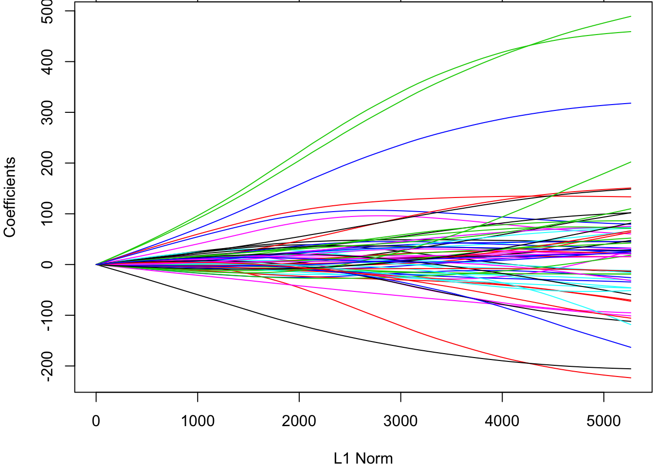
Cross-validation to tune the shrinkage parameter.
> cvridgefit <- glmnetUtils::cv.glmnet(y ~ ., data=df, alpha=0)
> plot(cvridgefit)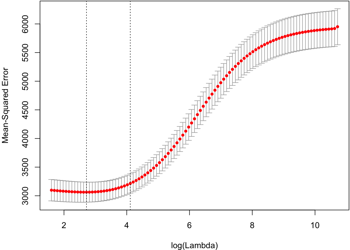
75.13 GLMs
The glmnet library (and the glmnetUtils wrapper library) allow one to perform ridge regression on generalized linear models.
A penalized maximum likelihood estimate is calculated based on
\[ -\lambda \sum_{i=1}^m \beta_i^2 \]
added to the log-likelihood.