12 Random Variables
12.1 Definition
A random variable \(X\) is a function from \(\Omega\) to the real numbers:
\[X: \Omega \rightarrow \mathbb{R}\]
For any outcome in \(\Omega\), the function \(X(\omega)\) produces a real value.
We will write the range of \(X\) as
\[\mathcal{R} = \{X(\omega): \omega \in \Omega\}\]
where \(\mathcal{R} \subseteq \mathbb{R}\).
12.2 Distributon of RV
We define the probability distribution of a random variable through its probability mass function (pmf) for discrete rv’s or its probability density function (pdf) for continuous rv’s.
We can also define the distribution through its cumulative distribution function (cdf). The pmf/pdf determines the cdf, and vice versa.
12.3 Discrete Random Variables
A discrete rv \(X\) takes on a discrete set of values such as \(\{1, 2, \ldots, n\}\) or \(\{0, 1, 2, 3, \ldots \}\).
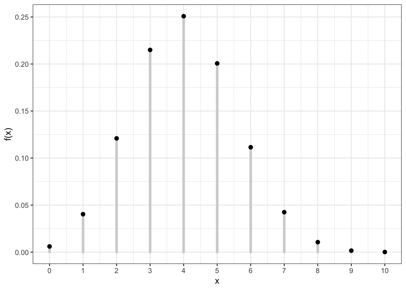
Its distribution is characterized by its pmf \[f(x) = \Pr(X = x)\] for \(x \in \{X(\omega): \omega \in \Omega \}\) and \(f(x) = 0\) otherwise.
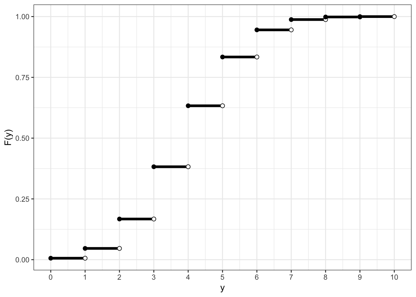
Its cdf is \[F(y) = \Pr(X \leq y) = \sum_{x \leq y} \Pr(X = x)\] for \(y \in \mathbb{R}\).
12.4 Example: Discrete PMF
12.5 Example: Discrete CDF
12.6 Probabilities of Events Via Discrete CDF
Examples:
| Probability | CDF | PMF |
|---|---|---|
| \(\Pr(X \leq b)\) | \(F(b)\) | \(\sum_{x \leq b} f(x)\) |
| \(\Pr(X \geq a)\) | \(1-F(a-1)\) | \(\sum_{x \geq a} f(x)\) |
| \(\Pr(X > a)\) | \(1-F(a)\) | \(\sum_{x > a} f(x)\) |
| \(\Pr(a \leq X \leq b)\) | \(F(b) - F(a-1)\) | \(\sum_{a \leq x \leq b} f(x)\) |
| \(\Pr(a < X \leq b)\) | \(F(b) - F(a)\) | \(\sum_{a < x \leq b} f(x)\) |
12.7 Continuous Random Variables
A continuous rv \(X\) takes on a continuous set of values such as \([0, \infty)\) or \(\mathbb{R} = (-\infty, \infty)\).
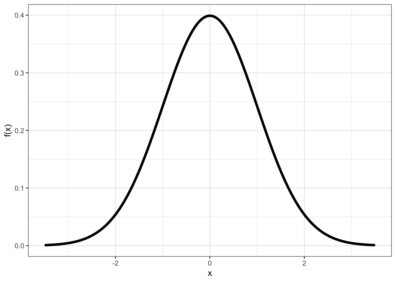
The probability that \(X\) takes on any specific value is 0; but the probability it lies within an interval can be non-zero. Its pdf \(f(x)\) therefore gives an infinitesimal, local, relative probability.
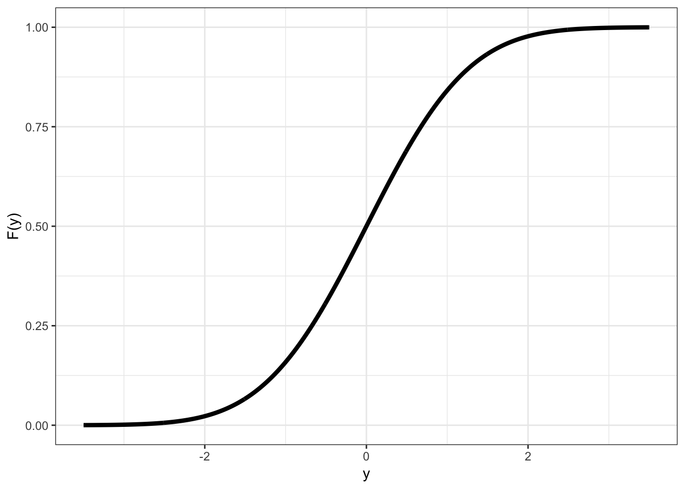
Its cdf is \[F(y) = \Pr(X \leq y) = \int_{-\infty}^y f(x) dx\] for \(y \in \mathbb{R}\).
12.8 Example: Continuous PDF
12.9 Example: Continuous CDF
12.10 Probabilities of Events Via Continuous CDF
Examples:
| Probability | CDF | |
|---|---|---|
| \(\Pr(X \leq b)\) | \(F(b)\) | \(\int_{-\infty}^{b} f(x) dx\) |
| \(\Pr(X \geq a)\) | \(1-F(a)\) | \(\int_{a}^{\infty} f(x) dx\) |
| \(\Pr(X > a)\) | \(1-F(a)\) | \(\int_{a}^{\infty} f(x) dx\) |
| \(\Pr(a \leq X \leq b)\) | \(F(b) - F(a)\) | \(\int_{a}^{b} f(x) dx\) |
| \(\Pr(a < X \leq b)\) | \(F(b) - F(a)\) | \(\int_{a}^{b} f(x) dx\) |
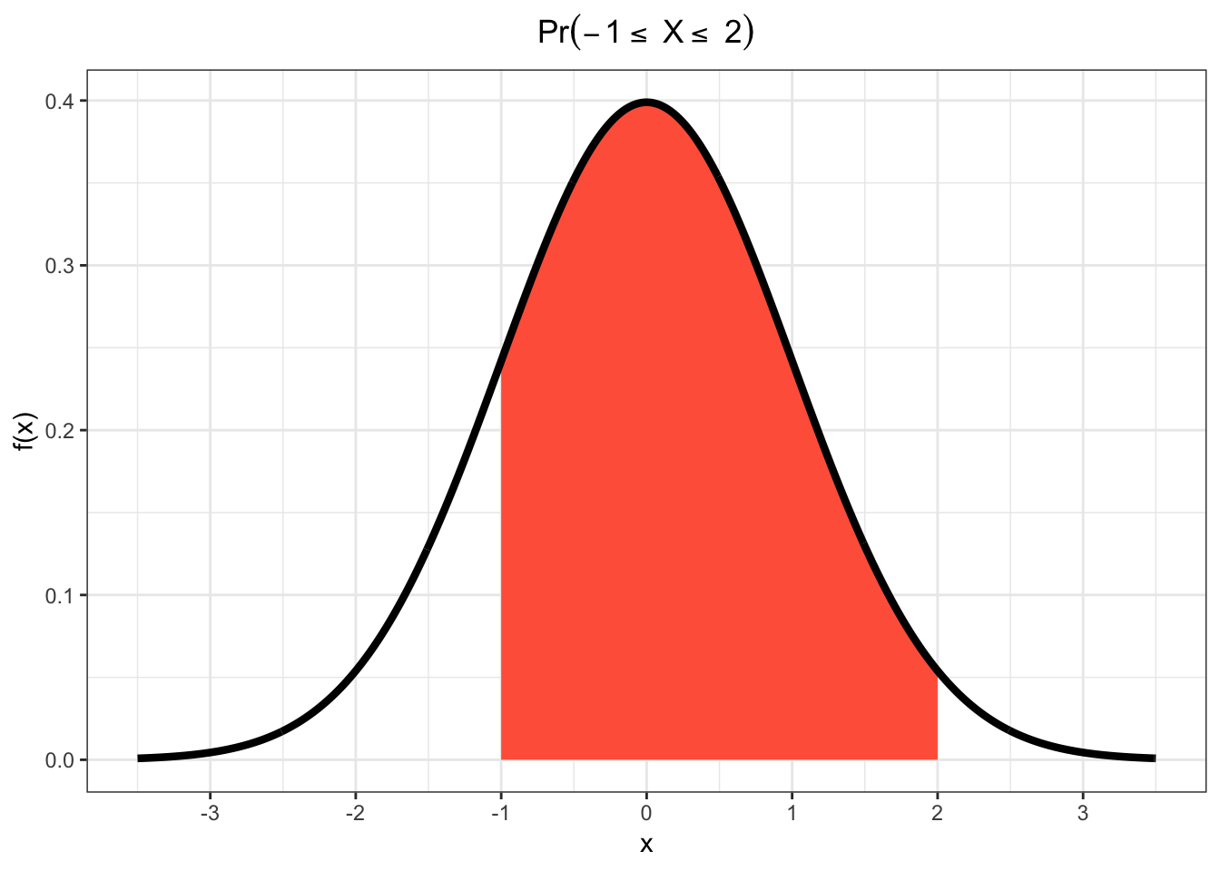
12.11 Example: Continuous RV Event
12.12 Note on PMFs and PDFs
PMFs and PDFs are defined as \(f(x)=0\) outside of the range of \(X\), \(\mathcal{R} = \{X(\omega): \omega \in \Omega\}\). That is:
Also, they sum or integrate to 1:
\[\sum_{x \in \mathcal{R}} f(x) = 1\]
\[\int_{x \in \mathcal{R}} f(x) dx = 1\]
Using measure theory, we can consider both types of rv’s in one framework, and we would write: \[\int_{-\infty}^{\infty} dF(x) = 1\]
12.13 Note on CDFs
Properties of all cdf’s, regardless of continuous or discrete underlying rv:
- They are right continuous with left limits
- \(\lim_{x \rightarrow \infty} F(x) = 1\)
- \(\lim_{x \rightarrow -\infty} F(x) = 0\)
- The right derivative of \(F(x)\) equals \(f(x)\)
12.14 Sample Vs Population Statistics
We earlier discussed measures of center and spread for a set of data, such as the mean and the variance.
Analogous measures exist for probability distributions.
These are distinguished by calling those on data “sample” measures (e.g., sample mean) and those on probability distributions “population” measures (e.g., population mean).
12.15 Expected Value
The expected value, also called the “population mean”, is a measure of center for a rv. It is calculated in a fashion analogous to the sample mean:
\[\begin{align*} & \operatorname{E}[X] = \sum_{x \in \mathcal{R}} x \ f(x) & \mbox{(discrete)} \\ & \operatorname{E}[X] = \int_{-\infty}^{\infty} x \ f(x) \ dx & \mbox{(continuous)} \\ & \operatorname{E}[X] = \int_{-\infty}^{\infty} x \ dF(x) & \mbox{(general)} \end{align*}\]12.16 Variance
The variance, also called the “population variance”, is a measure of spread for a rv. It is calculated in a fashion analogous to the sample variance:
\[{\operatorname{Var}}(X) = {\operatorname{E}}\left[\left(X-{\operatorname{E}}[X]\right)^2\right] = {\operatorname{E}}[X^2] - E[X]^2\] \[{\rm SD}(X) = \sqrt{{\operatorname{Var}}(X)}\]
\[{\operatorname{Var}}(X) = \sum_{x \in \mathcal{R}} \left(x-{\operatorname{E}}[X]\right)^2 \ f(x) \ \ \ \ \mbox{(discrete)}\]
\[{\operatorname{Var}}(X) = \int_{-\infty}^{\infty} \left(x-{\operatorname{E}}[X]\right)^2 \ f(x) \ dx \ \ \ \ \mbox{(continuous)}\]
12.17 Moment Generating Functions
The moment generating function (mgf) of a rv is defined to be
\[m(t) = \operatorname{E}\left[e^{tX}\right]\]
whenever this expecation exists.
Under certain conditions, the moments of a rv can then be obtained by:
\[\operatorname{E} \left[ X^k \right] = \frac{d^k}{dt^k}m(0).\]
12.18 Random Variables in R
The pmf/pdf, cdf, quantile function, and random number generator for many important random variables are built into R. They all follow the form, where <name> is replaced with the name used in R for each specific distribution:
d<name>: pmf or pdfp<name>: cdfq<name>: quantile function or inverse cdfr<name>: random number generator
To see a list of random variables, type ?Distributions in R.