30 Inference in R

30.1 BSDA Package

> install.packages("BSDA")

> library(BSDA)
> str(z.test)
function (x, y = NULL, alternative = "two.sided", mu = 0, sigma.x = NULL, 
    sigma.y = NULL, conf.level = 0.95)  

30.2 Example: Poisson

Apply z.test():

> set.seed(210)

> n <- 40
> lam <- 14
> x <- rpois(n=n, lambda=lam)
> lam.hat <- mean(x)
> stddev <- sqrt(lam.hat)
> z.test(x=x, sigma.x=stddev, mu=lam)

    One-sample z-Test

data:  x
z = 0.41885, p-value = 0.6753
alternative hypothesis: true mean is not equal to 14
95 percent confidence interval:
 13.08016 15.41984
sample estimates:
mean of x 
    14.25 

30.3 Direct Calculations

Confidence interval:

> lam.hat <- mean(x)
> lam.hat
[1] 14.25
> stderr <- sqrt(lam.hat)/sqrt(n)
> lam.hat - abs(qnorm(0.025)) * stderr # lower bound
[1] 13.08016
> lam.hat + abs(qnorm(0.025)) * stderr # upper bound
[1] 15.41984

Hypothesis test:

> z <- (lam.hat - lam)/stderr
> z # test statistic
[1] 0.4188539
> 2 * pnorm(-abs(z)) # two-sided p-value
[1] 0.6753229

30.4 Commonly Used Functions

R has the following functions for doing inference on some of the distributions we have considered.

• Normal: t.test()
• Binomial: binomial.test() or prop.test()
• Poisson: poisson.test()

These perform one-sample and two-sample hypothesis testing and confidence interval construction for both the one-sided and two-sided cases.

30.5 About These Functions

• We covered a convenient, unified MLE framework that allows us to better understand how confidence intervals and hypothesis testing are performed

• However, this framework requires large sample sizes and is not necessarily the best method to apply in all circumstances

• The above R functions are versatile functions for analyzing Normal, Binomial, and Poisson distributed data (or approximations thereof) that use much broader theory and methods than we have covered

• However, the arguments these functions take and the ouput of the functions are in line with the framework that we have covered

30.6 Normal Data: “Davis” Data Set

> library("car")
> data("Davis")

> htwt <- tbl_df(Davis)
> htwt
# A tibble: 200 x 5
   sex   weight height repwt repht
   <fct>  <int>  <int> <int> <int>
 1 M         77    182    77   180
 2 F         58    161    51   159
 3 F         53    161    54   158
 4 M         68    177    70   175
 5 F         59    157    59   155
 6 M         76    170    76   165
 7 M         76    167    77   165
 8 M         69    186    73   180
 9 M         71    178    71   175
10 M         65    171    64   170
# … with 190 more rows

30.7 Height vs Weight

> ggplot(htwt) + 
+ geom_point(aes(x=height, y=weight, color=sex), size=2, alpha=0.5) +
+ scale_colour_manual(values=c("red", "blue"))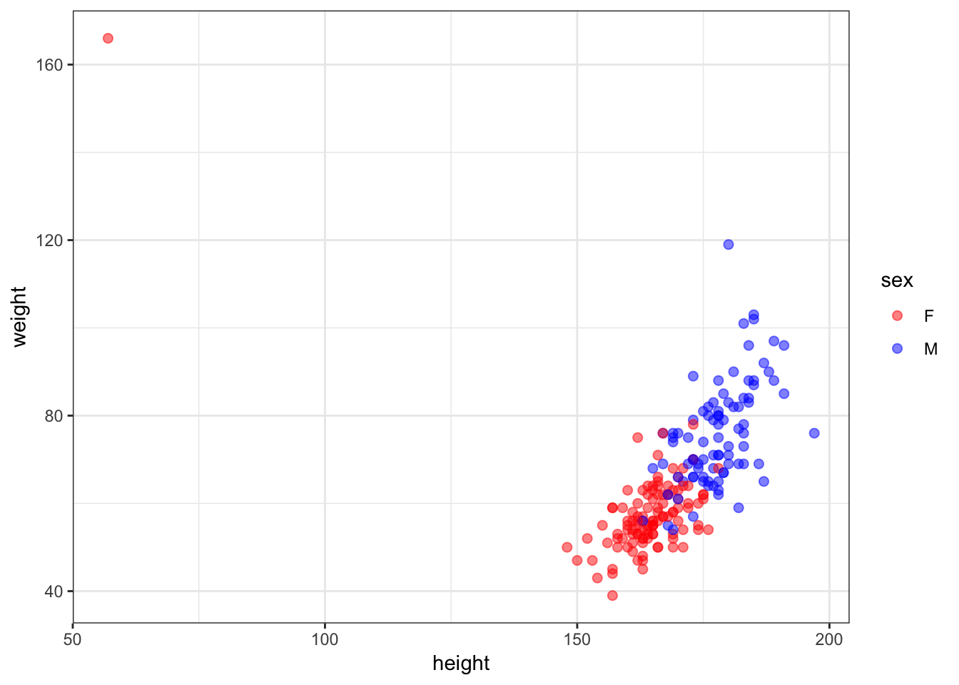

30.8 An Error?

> which(htwt$height < 100)
[1] 12
> htwt[12,]
# A tibble: 1 x 5
  sex   weight height repwt repht
  <fct>  <int>  <int> <int> <int>
1 F        166     57    56   163

> htwt[12,c(2,3)] <- htwt[12,c(3,2)]

30.9 Updated Height vs Weight

> ggplot(htwt) + 
+   geom_point(aes(x=height, y=weight, color=sex), size=2, alpha=0.5) +
+   scale_color_manual(values=c("red", "blue"))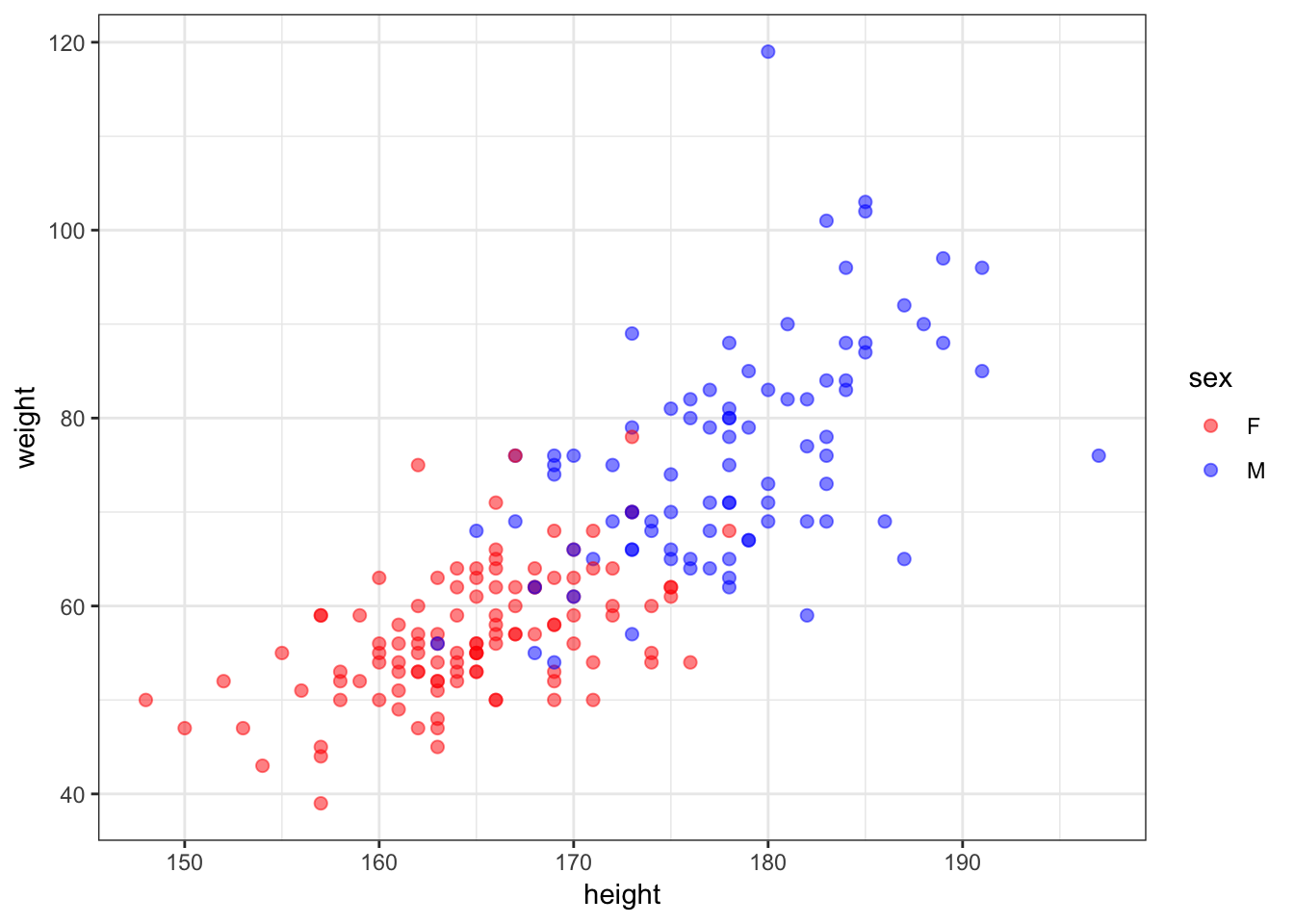

30.10 Density Plots of Height

> ggplot(htwt) + 
+   geom_density(aes(x=height, color=sex), size=1.5) + 
+   scale_color_manual(values=c("red", "blue"))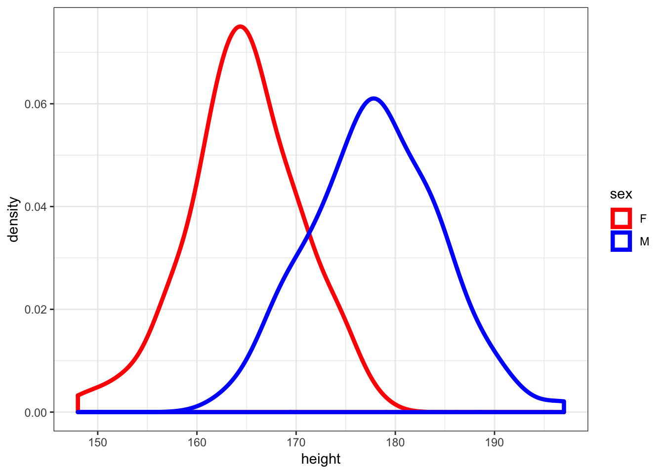

30.11 Density Plots of Weight

> ggplot(htwt) + 
+   geom_density(aes(x=weight, color=sex), size=1.5) + 
+   scale_color_manual(values=c("red", "blue"))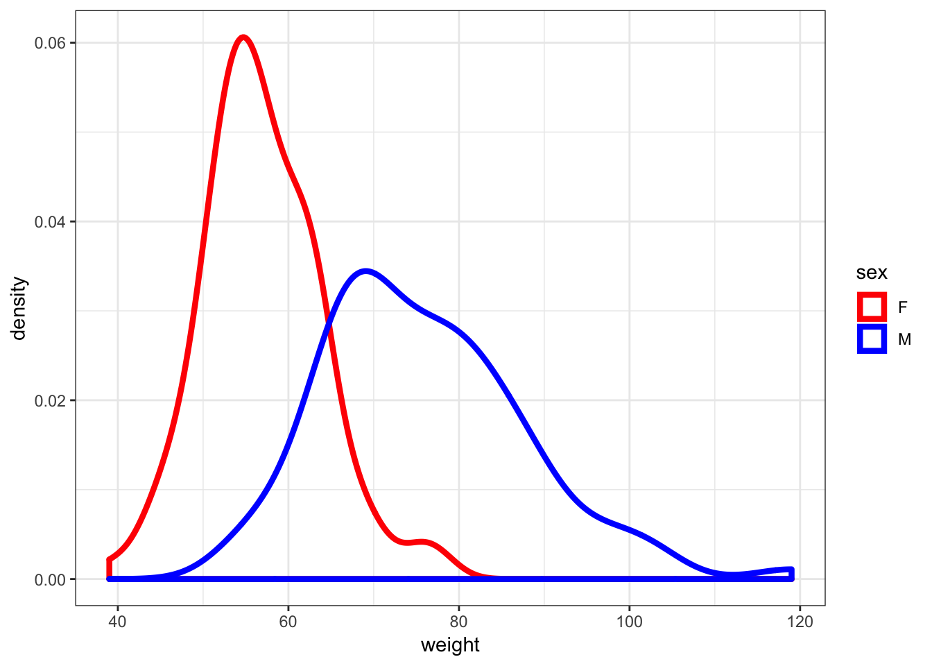

30.12 t.test() Function

From the help file…

Usage

t.test(x, ...)

## Default S3 method:
t.test(x, y = NULL,
       alternative = c("two.sided", "less", "greater"),
       mu = 0, paired = FALSE, var.equal = FALSE,
       conf.level = 0.95, ...)

## S3 method for class 'formula'
t.test(formula, data, subset, na.action, ...)

30.13 Two-Sided Test of Male Height

> m_ht <- htwt %>% filter(sex=="M") %>% select(height)
> testresult <- t.test(x = m_ht$height, mu=177)

> class(testresult)
[1] "htest"
> is.list(testresult)
[1] TRUE

30.14 Output of t.test()

> names(testresult)
 [1] "statistic"   "parameter"   "p.value"     "conf.int"    "estimate"   
 [6] "null.value"  "stderr"      "alternative" "method"      "data.name"  
> testresult

    One Sample t-test

data:  m_ht$height
t = 1.473, df = 87, p-value = 0.1443
alternative hypothesis: true mean is not equal to 177
95 percent confidence interval:
 176.6467 179.3760
sample estimates:
mean of x 
 178.0114 

30.15 Tidying the Output

> library(broom)
> tidy(testresult)
# A tibble: 1 x 8
  estimate statistic p.value parameter conf.low conf.high method
     <dbl>     <dbl>   <dbl>     <dbl>    <dbl>     <dbl> <chr> 
1     178.      1.47   0.144        87     177.      179. One S…
# … with 1 more variable: alternative <chr>

30.16 Two-Sided Test of Female Height

> f_ht <- htwt %>% filter(sex=="F") %>% select(height)
> t.test(x = f_ht$height, mu = 164)

    One Sample t-test

data:  f_ht$height
t = 1.3358, df = 111, p-value = 0.1844
alternative hypothesis: true mean is not equal to 164
95 percent confidence interval:
 163.6547 165.7739
sample estimates:
mean of x 
 164.7143 

30.17 Difference of Two Means

> t.test(x = m_ht$height, y = f_ht$height)

    Welch Two Sample t-test

data:  m_ht$height and f_ht$height
t = 15.28, df = 174.29, p-value < 2.2e-16
alternative hypothesis: true difference in means is not equal to 0
95 percent confidence interval:
 11.57949 15.01467
sample estimates:
mean of x mean of y 
 178.0114  164.7143 

30.18 Test with Equal Variances

> htwt %>% group_by(sex) %>% summarize(sd(height))
# A tibble: 2 x 2
  sex   `sd(height)`
  <fct>        <dbl>
1 F             5.66
2 M             6.44
> t.test(x = m_ht$height, y = f_ht$height, var.equal = TRUE)

    Two Sample t-test

data:  m_ht$height and f_ht$height
t = 15.519, df = 198, p-value < 2.2e-16
alternative hypothesis: true difference in means is not equal to 0
95 percent confidence interval:
 11.60735 14.98680
sample estimates:
mean of x mean of y 
 178.0114  164.7143 

30.19 Paired Sample Test (v. 1)

First take the difference between the paired observations. Then apply the one-sample t-test.

> htwt <- htwt %>% mutate(diffwt = (weight - repwt), 
+                         diffht = (height - repht))
> t.test(x = htwt$diffwt) %>% tidy()
# A tibble: 1 x 8
  estimate statistic p.value parameter conf.low conf.high method
     <dbl>     <dbl>   <dbl>     <dbl>    <dbl>     <dbl> <chr> 
1  0.00546    0.0319   0.975       182   -0.332     0.343 One S…
# … with 1 more variable: alternative <chr>
> t.test(x = htwt$diffht) %>% tidy()
# A tibble: 1 x 8
  estimate statistic  p.value parameter conf.low conf.high method
     <dbl>     <dbl>    <dbl>     <dbl>    <dbl>     <dbl> <chr> 
1     2.08      13.5 2.64e-29       182     1.77      2.38 One S…
# … with 1 more variable: alternative <chr>

30.20 Paired Sample Test (v. 2)

Enter each sample into the t.test() function, but use the paired=TRUE argument. This is operationally equivalent to the previous version.

> t.test(x=htwt$weight, y=htwt$repwt, paired=TRUE) %>% tidy()
# A tibble: 1 x 8
  estimate statistic p.value parameter conf.low conf.high method
     <dbl>     <dbl>   <dbl>     <dbl>    <dbl>     <dbl> <chr> 
1  0.00546    0.0319   0.975       182   -0.332     0.343 Paire…
# … with 1 more variable: alternative <chr>
> t.test(x=htwt$height, y=htwt$repht, paired=TRUE) %>% tidy()
# A tibble: 1 x 8
  estimate statistic  p.value parameter conf.low conf.high method
     <dbl>     <dbl>    <dbl>     <dbl>    <dbl>     <dbl> <chr> 
1     2.08      13.5 2.64e-29       182     1.77      2.38 Paire…
# … with 1 more variable: alternative <chr>
> htwt %>% select(height, repht) %>% na.omit() %>% 
+   summarize(mean(height), mean(repht))
# A tibble: 1 x 2
  `mean(height)` `mean(repht)`
           <dbl>         <dbl>
1           171.          168.

30.21 The Coin Flip Example

I flip it 20 times and it lands on heads 16 times.

1. My data is \(x=16\) heads out of \(n=20\) flips.
2. My data generation model is \(X \sim \mbox{Binomial}(20, p)\).
3. I form the statistic \(\hat{p} = 16/20\) as an estimate of \(p\).

Let’s do hypothesis testing and confidence interval construction on these data.

30.22 binom.test()

> str(binom.test)
function (x, n, p = 0.5, alternative = c("two.sided", "less", "greater"), 
    conf.level = 0.95)  
> binom.test(x=16, n=20, p = 0.5)

    Exact binomial test

data:  16 and 20
number of successes = 16, number of trials = 20, p-value = 0.01182
alternative hypothesis: true probability of success is not equal to 0.5
95 percent confidence interval:
 0.563386 0.942666
sample estimates:
probability of success 
                   0.8 

30.23 alternative = "greater"

Tests \(H_0: p \leq 0.5\) vs. \(H_1: p > 0.5\).

> binom.test(x=16, n=20, p = 0.5, alternative="greater")

    Exact binomial test

data:  16 and 20
number of successes = 16, number of trials = 20, p-value =
0.005909
alternative hypothesis: true probability of success is greater than 0.5
95 percent confidence interval:
 0.5989719 1.0000000
sample estimates:
probability of success 
                   0.8 

30.24 alternative = "less"

Tests \(H_0: p \geq 0.5\) vs. \(H_1: p < 0.5\).

> binom.test(x=16, n=20, p = 0.5, alternative="less")

    Exact binomial test

data:  16 and 20
number of successes = 16, number of trials = 20, p-value = 0.9987
alternative hypothesis: true probability of success is less than 0.5
95 percent confidence interval:
 0.0000000 0.9286461
sample estimates:
probability of success 
                   0.8 

30.25 prop.test()

This is a “large \(n\)” inference method that is very similar to our \(z\)-statistic approach.

> str(prop.test)
function (x, n, p = NULL, alternative = c("two.sided", "less", "greater"), 
    conf.level = 0.95, correct = TRUE)  
> prop.test(x=16, n=20, p=0.5)

    1-sample proportions test with continuity correction

data:  16 out of 20, null probability 0.5
X-squared = 6.05, df = 1, p-value = 0.01391
alternative hypothesis: true p is not equal to 0.5
95 percent confidence interval:
 0.5573138 0.9338938
sample estimates:
  p 
0.8 

30.26 An Observation

> p <- binom.test(x=16, n=20, p = 0.5)$p.value
> binom.test(x=16, n=20, p = 0.5, conf.level=(1-p))

    Exact binomial test

data:  16 and 20
number of successes = 16, number of trials = 20, p-value = 0.01182
alternative hypothesis: true probability of success is not equal to 0.5
98.81821 percent confidence interval:
 0.5000000 0.9625097
sample estimates:
probability of success 
                   0.8 

Exercise: Figure out what happened here.

30.27 Wording of Surveys

The way a question is phrased can influence a person’s response. For example, Pew Research Center conducted a survey with the following question:

“As you may know, by 2014 nearly all Americans will be required to have health insurance. [People who do not buy insurance will pay a penalty] while [People who cannot afford it will receive financial help from the government]. Do you approve or disapprove of this policy?”

For each randomly sampled respondent, the statements in brackets were randomized: either they were kept in the order given above, or the two statements were reversed.

Credit: This example comes from Open Intro Statistics, Exercise 6.10.

30.28 The Data

The following table shows the results of this experiment.

2nd Statement	Sample Size	Approve Law	Disapprove Law	Other
“people who cannot afford it will receive financial help from the government”	771	47	49	3
“people who do not buy it will pay a penalty”	732	34	63	3

30.29 Inference on the Difference

Create and interpret a 90% confidence interval of the difference in approval. Also perform a hyppthesis test that the approval rates are equal.

> x <- round(c(0.47*771, 0.34*732))
> n <- round(c(771*0.97, 732*0.97))
> prop.test(x=x, n=n, conf.level=0.90)

    2-sample test for equality of proportions with continuity
    correction

data:  x out of n
X-squared = 26.023, df = 1, p-value = 3.374e-07
alternative hypothesis: two.sided
90 percent confidence interval:
 0.08979649 0.17670950
sample estimates:
   prop 1    prop 2 
0.4839572 0.3507042 

30.30 90% Confidence Interval

Let’s use MLE theory to construct of a two-sided 90% CI.

> p1.hat <- 0.47
> n1 <- 771
> p2.hat <- 0.34
> n2 <- 732
> stderr <- sqrt(p1.hat*(1-p1.hat)/n1 + p2.hat*(1-p2.hat)/n2)
> 
> # the 90% CI
> (p1.hat - p2.hat) + c(-1,1)*abs(qnorm(0.05))*stderr
[1] 0.08872616 0.17127384

30.31 Poisson Data: poisson.test()

> str(poisson.test)
function (x, T = 1, r = 1, alternative = c("two.sided", "less", "greater"), 
    conf.level = 0.95)  

From the help:

Arguments

x    number of events. A vector of length one or two.

T    time base for event count. A vector of length one or two.

r    hypothesized rate or rate ratio

alternative  indicates the alternative hypothesis and must be one of 
"two.sided", "greater" or "less". You can specify just the initial letter.

conf.level  confidence level for the returned confidence interval.

30.32 Example: RNA-Seq

RNA-Seq gene expression was measured for p53 lung tissue in 12 healthy individuals and 14 individuals with lung cancer.

The counts were given as follows.

Healthy: 82 64 66 88 65 81 85 87 60 79 80 72

Cancer: 59 50 60 60 78 69 70 67 72 66 66 68 54 62

It is hypothesized that p53 expression is higher in healthy individuals. Test this hypothesis, and form a 99% CI.

30.33 \(H_1: \lambda_1 \not= \lambda_2\)

> healthy <- c(82, 64, 66, 88, 65, 81, 85, 87, 60, 79, 80, 72)
> cancer <- c(59, 50, 60, 60, 78, 69, 70, 67, 72, 66, 66, 68, 
+             54, 62)

> poisson.test(x=c(sum(healthy), sum(cancer)), T=c(12,14), 
+              conf.level=0.99)

    Comparison of Poisson rates

data:  c(sum(healthy), sum(cancer)) time base: c(12, 14)
count1 = 909, expected count1 = 835.38, p-value = 0.0005739
alternative hypothesis: true rate ratio is not equal to 1
99 percent confidence interval:
 1.041626 1.330051
sample estimates:
rate ratio 
  1.177026 

30.34 \(H_1: \lambda_1 < \lambda_2\)

> poisson.test(x=c(sum(healthy), sum(cancer)), T=c(12,14), 
+              alternative="less", conf.level=0.99)

    Comparison of Poisson rates

data:  c(sum(healthy), sum(cancer)) time base: c(12, 14)
count1 = 909, expected count1 = 835.38, p-value = 0.9998
alternative hypothesis: true rate ratio is less than 1
99 percent confidence interval:
 0.000000 1.314529
sample estimates:
rate ratio 
  1.177026 

30.35 \(H_1: \lambda_1 > \lambda_2\)

> poisson.test(x=c(sum(healthy), sum(cancer)), T=c(12,14), 
+              alternative="greater", conf.level=0.99)

    Comparison of Poisson rates

data:  c(sum(healthy), sum(cancer)) time base: c(12, 14)
count1 = 909, expected count1 = 835.38, p-value = 0.0002881
alternative hypothesis: true rate ratio is greater than 1
99 percent confidence interval:
 1.053921      Inf
sample estimates:
rate ratio 
  1.177026 

30.36 Question

Which analysis is the more informative and scientifically correct one, and why?