14 Continuous RVs

14.1 Uniform (Continuous)

Models the scenario where all values in the unit interval [0,1] are equally likely.

\[X \sim \mbox{Uniform}(0,1)\]

\[\mathcal{R} = [0,1]\]

\[f(x) = 1 \mbox{ for } x \in \mathcal{R}\]

\[F(y) = y \mbox{ for } y \in \mathcal{R}\]

\[{\operatorname{E}}[X] = 1/2, \ {\operatorname{Var}}(X) = 1/12\]

> str(dunif)
function (x, min = 0, max = 1, log = FALSE)

> str(punif)
function (q, min = 0, max = 1, lower.tail = TRUE, log.p = FALSE)

> str(qunif)
function (p, min = 0, max = 1, lower.tail = TRUE, log.p = FALSE)

> str(runif)
function (n, min = 0, max = 1)

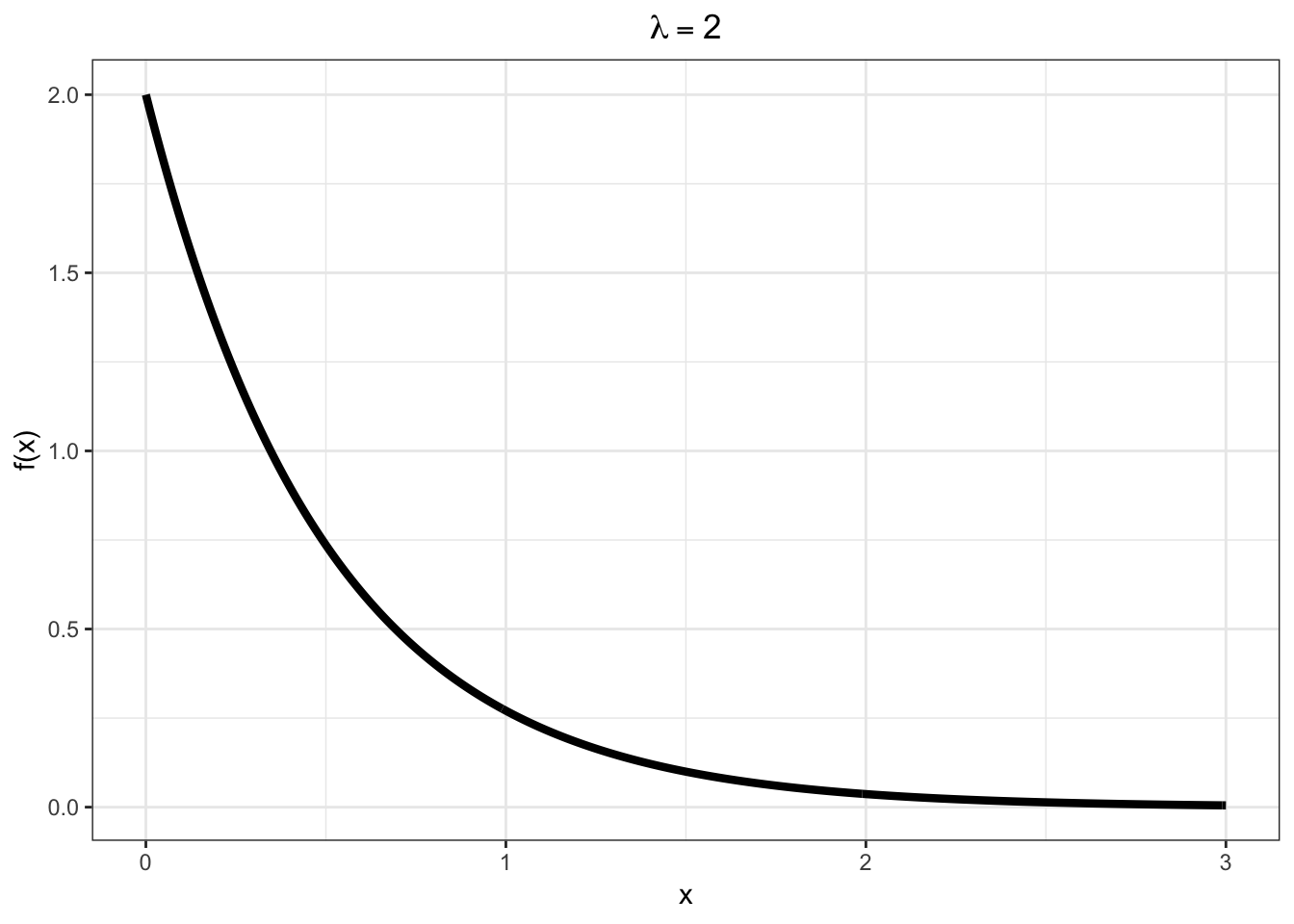
Models a time to failure and has a “memoryless property”.

\[X \sim \mbox{Exponential}(\lambda)\]

\[\mathcal{R} = [0, \infty)\]

\[f(x; \lambda) = \lambda e^{-\lambda x} \mbox{ for } x \in \mathcal{R}\]

\[F(y; \lambda) = 1 - e^{-\lambda y} \mbox{ for } y \in \mathcal{R}\]

\[{\operatorname{E}}[X] = \frac{1}{\lambda}, \ {\operatorname{Var}}(X) = \frac{1}{\lambda^2}\]

> str(dexp)
function (x, rate = 1, log = FALSE)

> str(pexp)
function (q, rate = 1, lower.tail = TRUE, log.p = FALSE)

> str(qexp)
function (p, rate = 1, lower.tail = TRUE, log.p = FALSE)

> str(rexp)
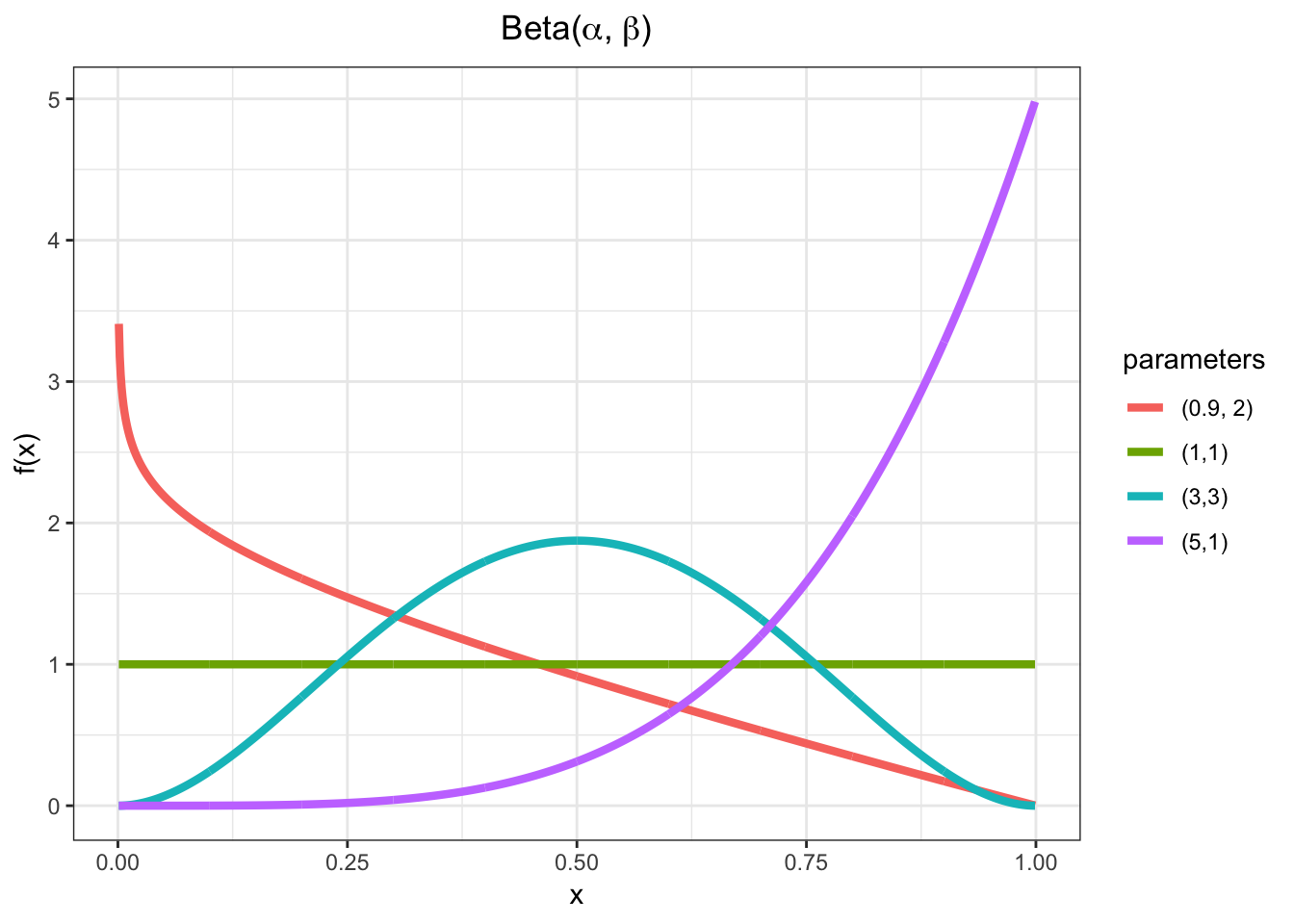
function (n, rate = 1)

Yields values in \((0,1)\), so often used to generate random probabilities, such as the \(p\) in Bernoulli\((p)\).

\[X \sim \mbox{Beta}(\alpha,\beta) \mbox{ where } \alpha, \beta > 0\]

\[\mathcal{R} = (0,1)\]

\[f(x; \alpha, \beta) = \frac{\Gamma(\alpha + \beta)}{\Gamma(\alpha) \Gamma(\beta)}x^{\alpha-1}(1-x)^{\beta - 1} \mbox{ for } x \in \mathcal{R}\]

where \(\Gamma(z) = \int_{0}^{\infty} x^{z-1} e^{-x} dx\).

\[{\operatorname{E}}[X] = \frac{\alpha}{\alpha + \beta}, \ {\operatorname{Var}}(X) = \frac{\alpha \beta}{(\alpha + \beta)^2 (\alpha + \beta + 1)}\]

> str(dbeta) #shape1=alpha, shape2=beta
function (x, shape1, shape2, ncp = 0, log = FALSE)

> str(pbeta)
function (q, shape1, shape2, ncp = 0, lower.tail = TRUE, log.p = FALSE)

> str(qbeta)
function (p, shape1, shape2, ncp = 0, lower.tail = TRUE, log.p = FALSE)

> str(rbeta)
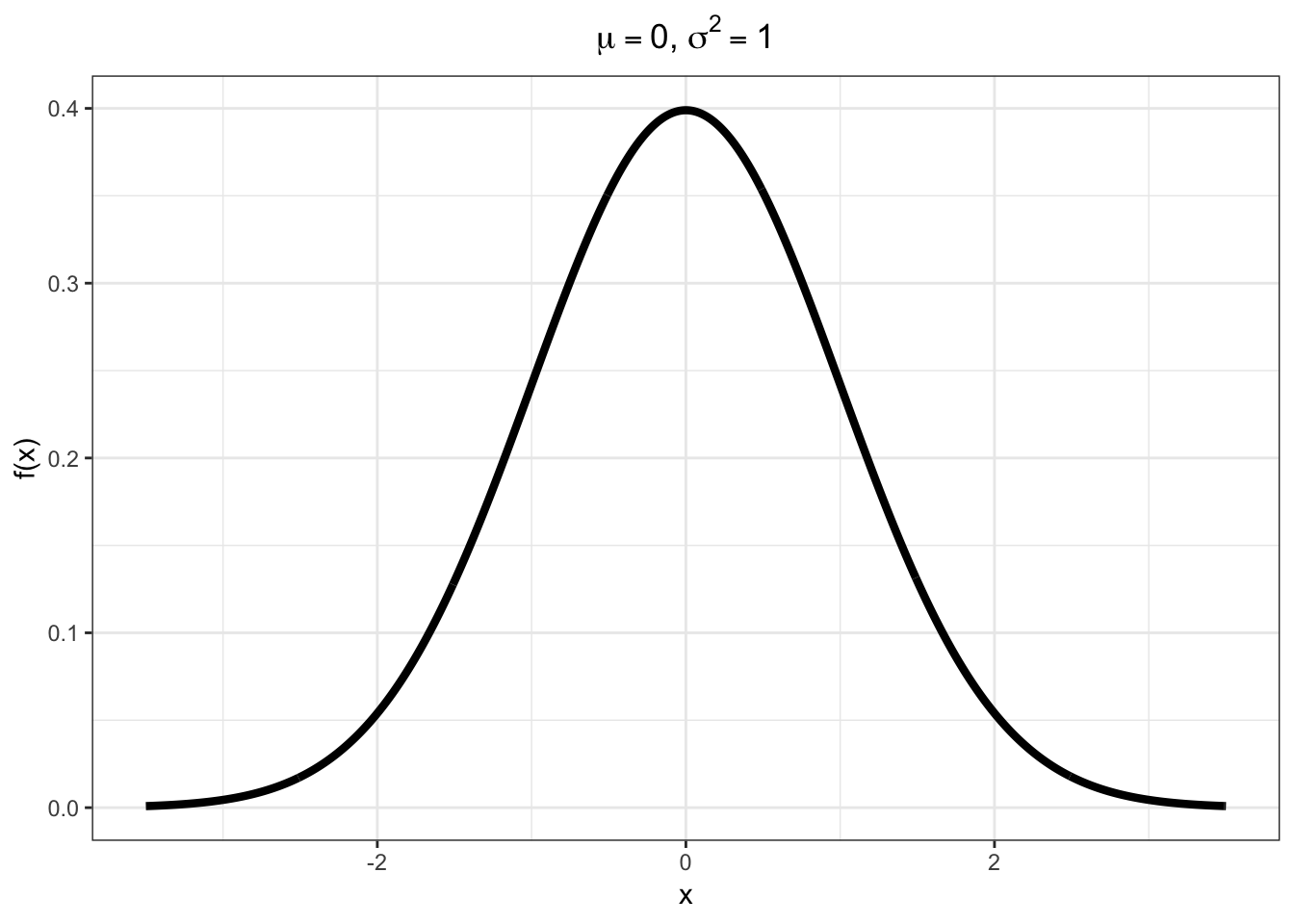
function (n, shape1, shape2, ncp = 0)

Due to the Central Limit Theorem (covered later), this “bell curve” distribution is often observed in properly normalized real data.

\[X \sim \mbox{Normal}(\mu, \sigma^2)\]

\[\mathcal{R} = (-\infty, \infty)\]

\[f(x; \mu, \sigma^2) = \frac{1}{\sqrt{2 \pi \sigma^2}} e^{-\frac{(x-\mu)^2}{2 \sigma^2}} \mbox{ for } x \in \mathcal{R}\]

\[{\operatorname{E}}[X] = \mu, \ {\operatorname{Var}}(X) = \sigma^2\]

> str(dnorm) #notice it requires the STANDARD DEVIATION, not the variance
function (x, mean = 0, sd = 1, log = FALSE)

> str(pnorm)
function (q, mean = 0, sd = 1, lower.tail = TRUE, log.p = FALSE)

> str(qnorm)
function (p, mean = 0, sd = 1, lower.tail = TRUE, log.p = FALSE)

> str(rnorm)
function (n, mean = 0, sd = 1)