57 lm() Function in R
57.1 Calculate the Line in R
The syntax for a model in R is
response variable ~ explanatory variables
where the explanatory variables component can involve several types of terms.
> myfit <- lm(weight ~ height, data=htwt)
> myfit

Call:
lm(formula = weight ~ height, data = htwt)

Coefficients:
(Intercept)       height
    -130.91         1.15
57.2 An lm Object is a List
> class(myfit)
[1] "lm"
> is.list(myfit)
[1] TRUE
> names(myfit)
 [1] "coefficients"  "residuals"     "effects"       "rank"
 [5] "fitted.values" "assign"        "qr"            "df.residual"
 [9] "xlevels"       "call"          "terms"         "model"
57.3 From the R Help
lmreturns an object of class “lm” or for multiple responses of class c(“mlm”, “lm”).
The functions
summaryandanovaare used to obtain and print a summary and analysis of variance table of the results. The generic accessor functions coefficients, effects, fitted.values and residuals extract various useful features of the value returned bylm.
57.4 Some of the List Items
These are some useful items to access from the lm object:
coefficients: a named vector of coefficientsresiduals: the residuals, that is response minus fitted values.fitted.values: the fitted mean values.df.residual: the residual degrees of freedom.call: the matched call.model: if requested (the default), the model frame used.
57.5 summary()
> summary(myfit)

Call:
lm(formula = weight ~ height, data = htwt)

Residuals:
    Min      1Q  Median      3Q     Max
-19.658  -5.381  -0.555   4.807  42.894

Coefficients:
              Estimate Std. Error t value Pr(>|t|)
(Intercept) -130.91040   11.52792  -11.36   <2e-16 ***
height         1.15009    0.06749   17.04   <2e-16 ***
---
Signif. codes:  0 '***' 0.001 '**' 0.01 '*' 0.05 '.' 0.1 ' ' 1

Residual standard error: 8.505 on 198 degrees of freedom
Multiple R-squared:  0.5946,    Adjusted R-squared:  0.5925
F-statistic: 290.4 on 1 and 198 DF,  p-value: < 2.2e-16
57.6 summary() List Elements
> mysummary <- summary(myfit)
> names(mysummary)
 [1] "call"          "terms"         "residuals"     "coefficients"
 [5] "aliased"       "sigma"         "df"            "r.squared"
 [9] "adj.r.squared" "fstatistic"    "cov.unscaled"
57.7 Using tidy()
> library(broom)
> tidy(myfit)
# A tibble: 2 x 5
  term        estimate std.error statistic  p.value
  <chr>          <dbl>     <dbl>     <dbl>    <dbl>
1 (Intercept)  -131.     11.5        -11.4 2.44e-23
2 height          1.15    0.0675      17.0 1.12e-40
57.8 Proportion of Variation Explained
The proportion of variance explained by the fitted model is called \(R^2\) or \(r^2\). It is calculated by:
\[r^2 = \frac{s^2_{\hat{y}}}{s^2_{y}}\]
> summary(myfit)$r.squared
[1] 0.5945555
>
> var(myfit$fitted.values)/var(htwt$weight)
[1] 0.5945555
57.9 Assumptions to Verify
The assumptions on the above linear model are really about the joint distribution of the residuals, which are not directly observed. On data, we try to verify:
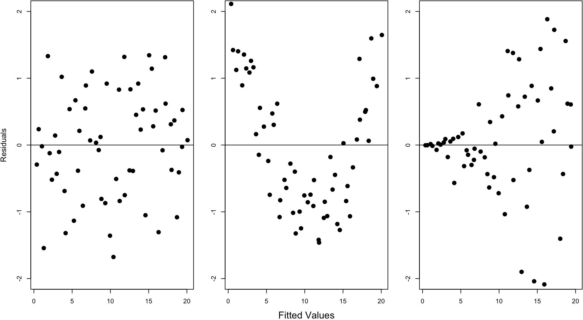
- The fitted values and the residuals show no trends with respect to each other
- The residuals are distributed approximately Normal\((0, \sigma^2)\)
- A constant variance is called homoscedasticity
- A non-constant variance is called heteroscedascity
- There are no lurking variables
There are two plots we will use in this course to investigate the first two.
57.10 Residual Distribution
> plot(myfit, which=1)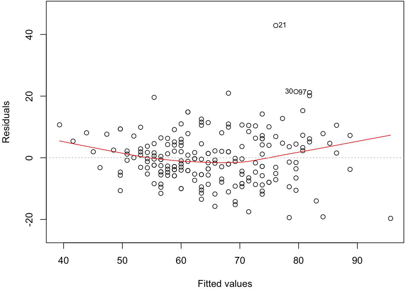
57.11 Normal Residuals Check
> plot(myfit, which=2)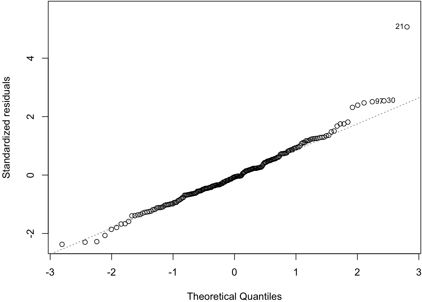
57.12 Fitted Values Vs. Obs. Residuals