29 The t Distribution
29.1 Normal, Unknown Variance
Suppose a sample of \(n\) data points is modeled by \(X_1, X_2, \ldots, X_n \stackrel{{\rm iid}}{\sim} \mbox{Normal}(\mu, \sigma^2)\) where \(\sigma^2\) is unknown. Recall that \(S = \sqrt{\frac{\sum_{i=1}^n (X_i - \overline{X})^2}{n-1}}\) is the sample standard deviation.
The statistic \[\frac{\overline{X} - \mu}{S/\sqrt{n}}\]
has a \(t_{n-1}\) distribution, a t-distribution with \(n-1\) degrees of freedom.
29.2 Aside: Chi-Square Distribution
Suppose \(Z_1, Z_2, \ldots, Z_v \stackrel{{\rm iid}}{\sim} \mbox{Normal}(0, 1)\). Then \(Z_1^2 + Z_2^2 + \cdots + Z_v^2\) has a \(\chi^2_v\) distribution, where \(v\) is the degrees of freedom.
This \(\chi^2_v\) rv has a pdf, expected value equal to \(v\), and variance equal to \(2v\).
Also,
\[\frac{(n-1) S^2}{\sigma^2} \sim \chi^2_{n-1}.\]
29.3 Theoretical Basis of the t
Suppose that \(Z \sim \mbox{Normal}(0,1)\), \(X \sim \chi^2_v\), and \(Z\) and \(X\) are independent. Then \(\frac{Z}{\sqrt{X/v}}\) has a \(t_v\) distribution.
Since \(\frac{\overline{X} - \mu}{\sigma/\sqrt{n}} \sim \mbox{Normal}(0,1)\) and \(\overline{X}\) and \(S^2\) are independent (shown later), it follows that the following has a \(t_{n-1}\) distribution:
\[\frac{\overline{X} - \mu}{S/\sqrt{n}}.\]
29.4 When Is t Utilized?
- The t distribution and its corresponding CI’s and HT’s are utilized when the data are Normal (or approximately Normal) and \(n\) is small
- Small typically means that \(n < 30\)
- In this case the inference based on the t distribution will be more accurate
- When \(n \geq 30\), there is very little difference between using \(t\)-statistics and \(z\)-statistics
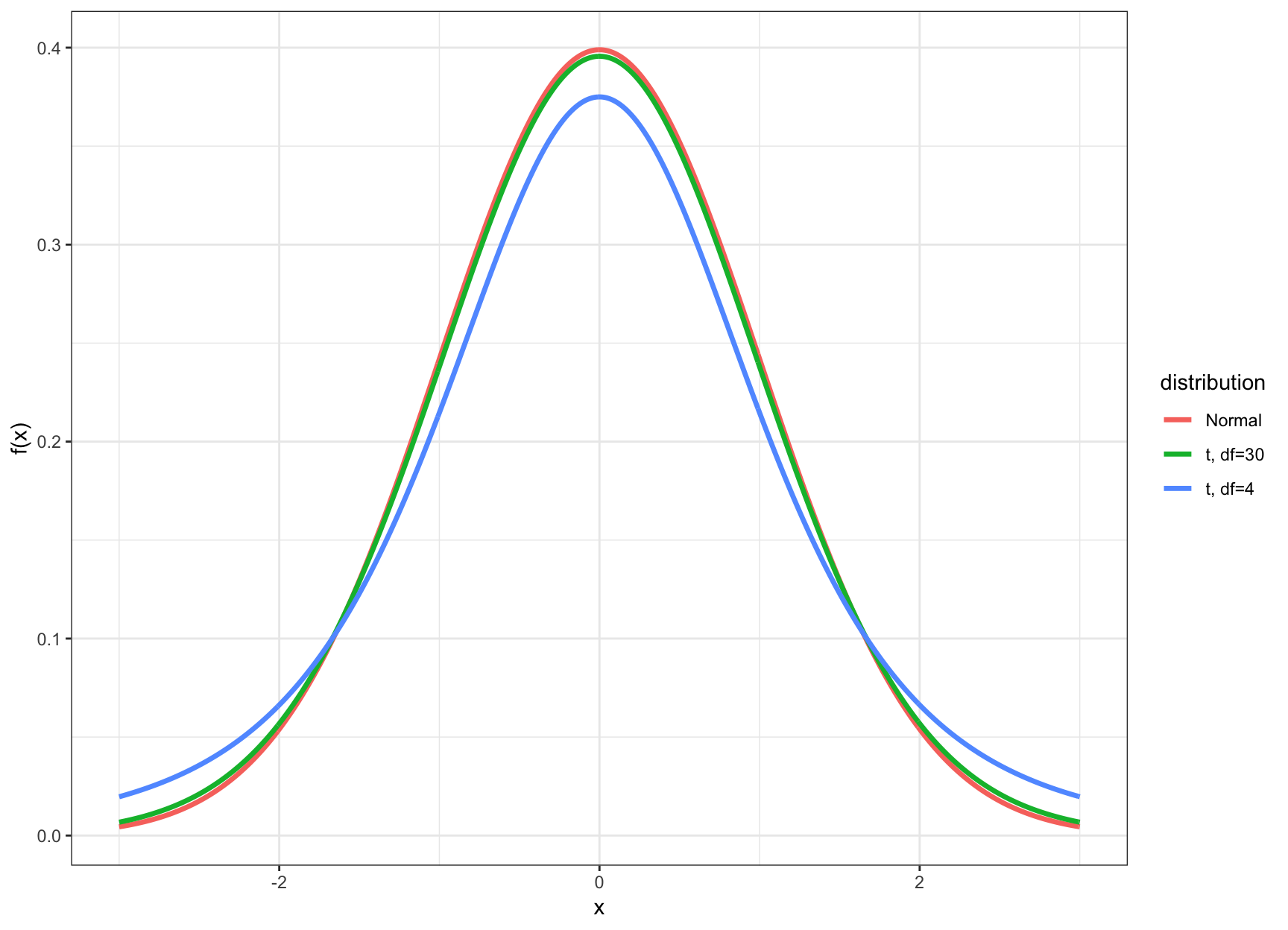
29.5 t vs Normal
29.6 t Percentiles
We calculated percentiles of the Normal(0,1) distribution (e.g., \(z_\alpha\)). We can do the analogous calculation with the t distribution.
Let \(t_\alpha\) be the \(\alpha\) percentile of the t distribution. Examples:
> qt(0.025, df=4) # alpha = 0.025
[1] -2.776445
> qt(0.05, df=4)
[1] -2.131847
> qt(0.95, df=4)
[1] 2.131847
> qt(0.975, df=4)
[1] 2.776445
29.7 Confidence Intervals
Here is a \((1-\alpha)\)-level CI for \(\mu\) using this distribution:
\[ \left(\hat{\mu} - |t_{\alpha/2}| \frac{s}{\sqrt{n}}, \hat{\mu} + |t_{\alpha/2}| \frac{s}{\sqrt{n}} \right), \]
where as before \(\hat{\mu} = \overline{x}\). This produces a wider CI than the \(z\) statistic analogue.
29.8 Hypothesis Tests
Suppose we want to test \(H_0: \mu = \mu_0\) vs \(H_1: \mu \not= \mu_0\) where \(\mu_0\) is a known, given number.
The t-statistic is
\[ t = \frac{\hat{\mu} - \mu_0}{\frac{s}{\sqrt{n}}} \]
with p-value
\[ {\rm Pr}(|T^*| \geq |t|) \]
where \(T^* \sim t_{n-1}\).
29.9 Two-Sample t-Distribution
Let \(X_1, X_2, \ldots, X_{n_1} \stackrel{{\rm iid}}{\sim} \mbox{Normal}(\mu_1, \sigma^2_1)\) and \(Y_1, Y_2, \ldots, Y_{n_2} \stackrel{{\rm iid}}{\sim} \mbox{Normal}(\mu_2, \sigma^2_2)\) have unequal variances.
We have \(\hat{\mu}_1 = \overline{X}\) and \(\hat{\mu}_2 = \overline{Y}\). The unequal variance two-sample t-statistic is \[ t = \frac{\hat{\mu}_1 - \hat{\mu}_2 - (\mu_1 - \mu_2)}{\sqrt{\frac{S^2_1}{n_1} + \frac{S^2_2}{n_2}}}. \]
29.10 Two-Sample t-Distribution
Let \(X_1, X_2, \ldots, X_{n_1} \stackrel{{\rm iid}}{\sim} \mbox{Normal}(\mu_1, \sigma^2)\) and \(Y_1, Y_2, \ldots, Y_{n_2} \stackrel{{\rm iid}}{\sim} \mbox{Normal}(\mu_2, \sigma^2)\) have equal variance.
We have \(\hat{\mu}_1 = \overline{X}\) and \(\hat{\mu}_2 = \overline{Y}\). The equal variance two-sample t-statistic is
\[ t = \frac{\hat{\mu}_1 - \hat{\mu}_2 - (\mu_1 - \mu_2)}{\sqrt{\frac{S^2}{n_1} + \frac{S^2}{n_2}}}. \]
where
\[ S^2 = \frac{\sum_{i=1}^{n_1}(X_i - \overline{X})^2 + \sum_{i=1}^{n_2}(Y_i - \overline{Y})^2}{n_1 + n_2 - 2}. \]
29.11 Two-Sample t-Distributions
When the two populations have equal variances, the pivotal t-statistic follows a \(t_{n_1 + n_2 -2}\) distribution.
When there are unequal variances, the pivotal t-statistic follows a t distribution where the degrees of freedom comes from an approximation using the Welch–Satterthwaite equation (which R calculates).