61 Categorical Explanatory Variables
61.1 Example: Chicken Weights
> data("chickwts", package="datasets")
> head(chickwts)
  weight      feed
1    179 horsebean
2    160 horsebean
3    136 horsebean
4    227 horsebean
5    217 horsebean
6    168 horsebean
> summary(chickwts$feed)
   casein horsebean   linseed  meatmeal   soybean sunflower
       12        10        12        11        14        12
61.2 Factor Variables in lm()
> chick_fit <- lm(weight ~ feed, data=chickwts)
> summary(chick_fit)

Call:
lm(formula = weight ~ feed, data = chickwts)

Residuals:
     Min       1Q   Median       3Q      Max
-123.909  -34.413    1.571   38.170  103.091

Coefficients:
              Estimate Std. Error t value Pr(>|t|)
(Intercept)    323.583     15.834  20.436  < 2e-16 ***
feedhorsebean -163.383     23.485  -6.957 2.07e-09 ***
feedlinseed   -104.833     22.393  -4.682 1.49e-05 ***
feedmeatmeal   -46.674     22.896  -2.039 0.045567 *
feedsoybean    -77.155     21.578  -3.576 0.000665 ***
feedsunflower    5.333     22.393   0.238 0.812495
---
Signif. codes:  0 '***' 0.001 '**' 0.01 '*' 0.05 '.' 0.1 ' ' 1

Residual standard error: 54.85 on 65 degrees of freedom
Multiple R-squared:  0.5417,    Adjusted R-squared:  0.5064
F-statistic: 15.36 on 5 and 65 DF,  p-value: 5.936e-10
61.3 Plot the Fit
> plot(chickwts$feed, chickwts$weight, xlab="Feed", ylab="Weight", las=2)
> points(chickwts$feed, chick_fit$fitted.values, col="blue", pch=20, cex=2)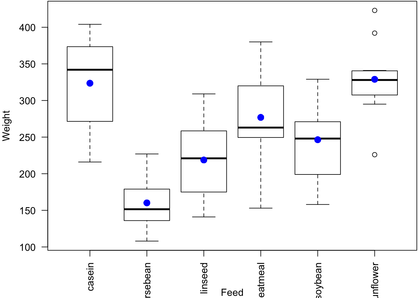
61.4 ANOVA (Version 1)
ANOVA (analysis of variance) was originally developed as a statistical model and method for comparing differences in mean values between various groups.
ANOVA quantifies and tests for differences in response variables with respect to factor variables.
In doing so, it also partitions the total variance to that due to within and between groups, where groups are defined by the factor variables.
61.5 anova()
The classic ANOVA table:
> anova(chick_fit)
Analysis of Variance Table

Response: weight
          Df Sum Sq Mean Sq F value    Pr(>F)
feed       5 231129   46226  15.365 5.936e-10 ***
Residuals 65 195556    3009
---
Signif. codes:  0 '***' 0.001 '**' 0.01 '*' 0.05 '.' 0.1 ' ' 1
> n <- length(chick_fit$residuals) # n <- 71
> (n-1)*var(chick_fit$fitted.values)
[1] 231129.2
> (n-1)*var(chick_fit$residuals)
[1] 195556
> (n-1)*var(chickwts$weight) # sum of above two quantities
[1] 426685.2
> (231129/5)/(195556/65) # F-statistic
[1] 15.3647961.6 How It Works
> levels(chickwts$feed)
[1] "casein"    "horsebean" "linseed"   "meatmeal"  "soybean"   "sunflower"
> head(chickwts, n=3)
  weight      feed
1    179 horsebean
2    160 horsebean
3    136 horsebean
> tail(chickwts, n=3)
   weight   feed
69    222 casein
70    283 casein
71    332 casein
> x <- model.matrix(weight ~ feed, data=chickwts)
> dim(x)
[1] 71  6
61.7 Top of Design Matrix
> head(x)
  (Intercept) feedhorsebean feedlinseed feedmeatmeal feedsoybean
1           1             1           0            0           0
2           1             1           0            0           0
3           1             1           0            0           0
4           1             1           0            0           0
5           1             1           0            0           0
6           1             1           0            0           0
  feedsunflower
1             0
2             0
3             0
4             0
5             0
6             0
61.8 Bottom of Design Matrix
> tail(x)
   (Intercept) feedhorsebean feedlinseed feedmeatmeal feedsoybean
66           1             0           0            0           0
67           1             0           0            0           0
68           1             0           0            0           0
69           1             0           0            0           0
70           1             0           0            0           0
71           1             0           0            0           0
   feedsunflower
66             0
67             0
68             0
69             0
70             0
71             0
61.9 Model Fits
> chick_fit$fitted.values %>% round(digits=4) %>% unique()
[1] 160.2000 218.7500 246.4286 328.9167 276.9091 323.5833
> chickwts %>% group_by(feed) %>% summarize(mean(weight))
# A tibble: 6 x 2
feed `mean(weight)`
<fct> <dbl>
1 casein 324.
2 horsebean 160.
3 linseed 219.
4 meatmeal 277.
5 soybean 246.
6 sunflower 329.