56 Simple Linear Regression

56.1 Definition

For random variables \((X_1, Y_1), (X_2, Y_2), \ldots, (X_n, Y_n)\), simple linear regression estimates the model

\[ Y_i = \beta_1 + \beta_2 X_i + E_i \]

where \({\operatorname{E}}[E_i] = 0\), \({\operatorname{Var}}(E_i) = \sigma^2\), and \({\operatorname{Cov}}(E_i, E_j) = 0\) for all \(1 \leq i, j \leq n\) and \(i \not= j\).

56.2 Rationale

Least squares linear regression is one of the simplest and most useful modeling systems for building a model that explains the variation of one variable in terms of other variables.
It is simple to fit, it satisfies some optimality criteria, and it is straightforward to check assumptions on the data so that statistical inference can be performed.

56.3 Setup

Suppose that we have observed \(n\) pairs of data \((x_1, y_1), (x_2, y_2), \ldots, (x_n, y_n)\).
Least squares linear regression models variation of the response variable \(y\) in terms of the explanatory variable \(x\) in the form of \(\beta_1 + \beta_2 x\), where \(\beta_1\) and \(\beta_2\) are chosen to satisfy a least squares optimization.

56.4 Line Minimizing Squared Error

The least squares regression line is formed from the value of \(\beta_1\) and \(\beta_2\) that minimize:

\[\sum_{i=1}^n \left( y_i - \beta_1 - \beta_2 x_i \right)^2.\]

For a given set of data, there is a unique solution to this minimization as long as there are at least two unique values among \(x_1, x_2, \ldots, x_n\).

Let \(\hat{\beta_1}\) and \(\hat{\beta_2}\) be the values that minimize this sum of squares.

56.5 Least Squares Solution

These values are:

\[\hat{\beta}_2 = r_{xy} \frac{s_y}{s_x}\]

\[\hat{\beta}_1 = \overline{y} - \hat{\beta}_2 \overline{x}\]

These values have a useful interpretation.

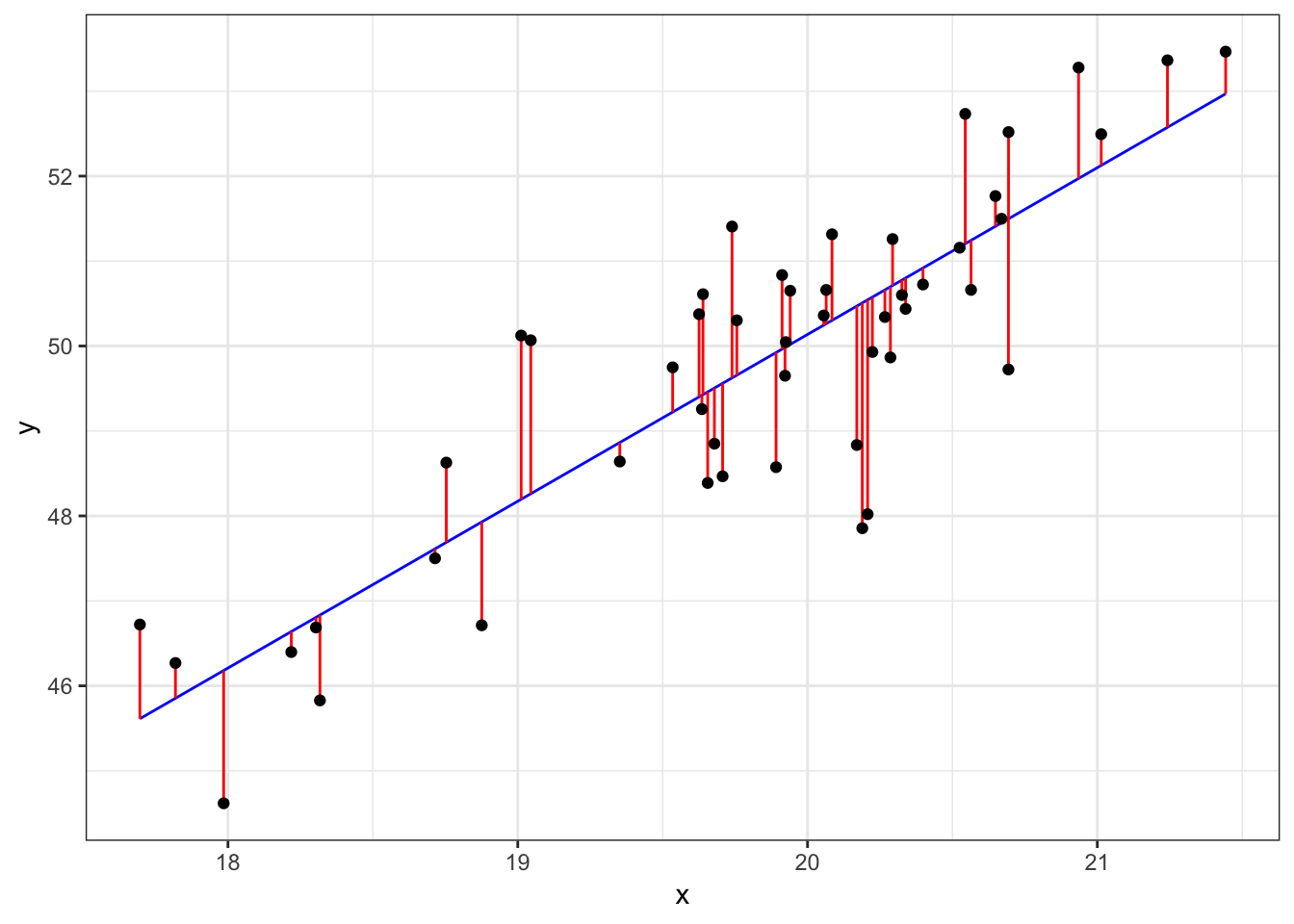
56.6 Visualizing Least Squares Line

56.7 Example: Height and Weight

> ggplot(data=htwt, mapping=aes(x=height, y=weight)) + 
+   geom_point(size=2, alpha=0.5) +
+   geom_smooth(method="lm", se=FALSE, formula=y~x)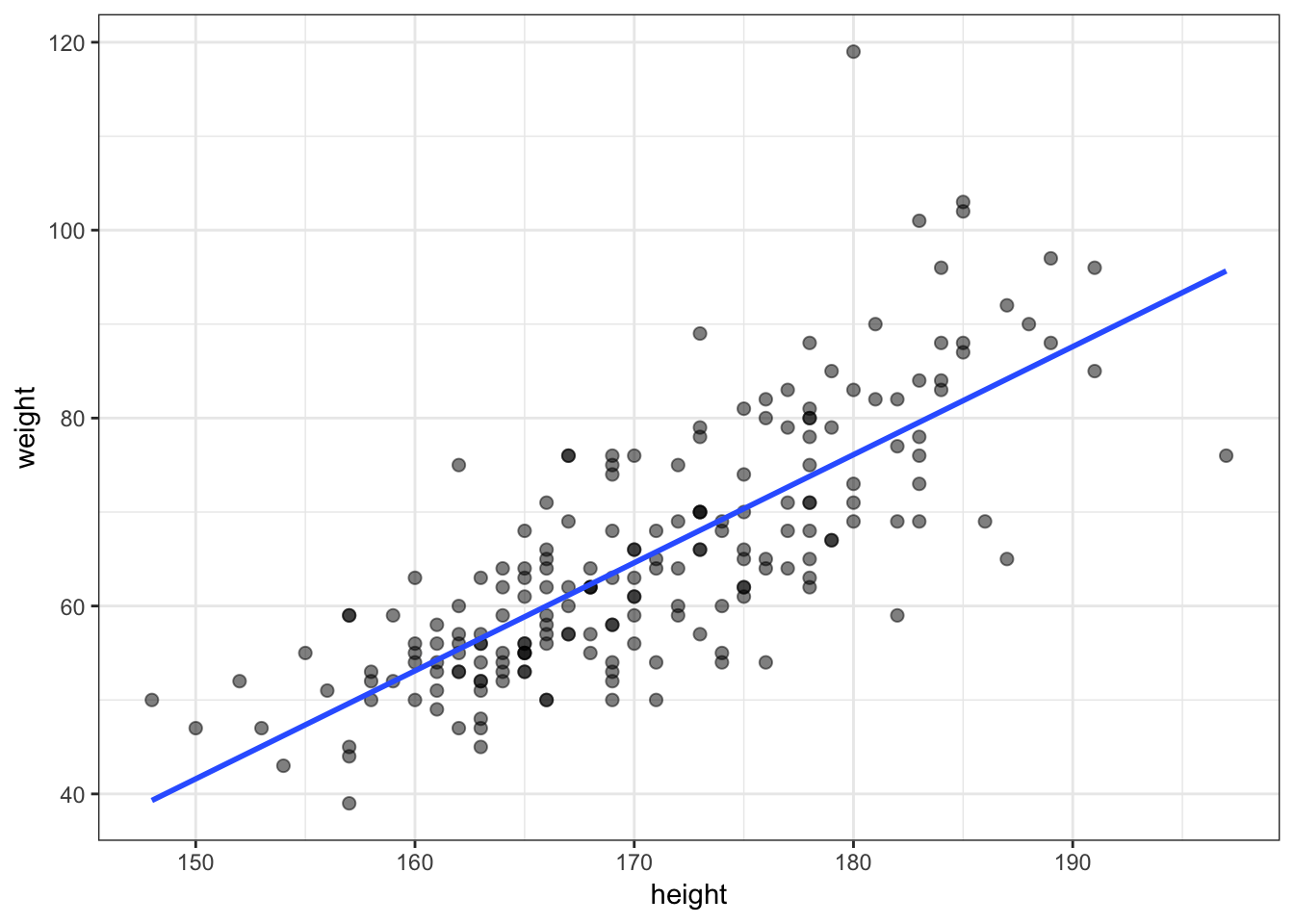

56.8 Calculate the Line Directly

> beta2 <- cor(htwt$height, htwt$weight) * 
+                sd(htwt$weight) / sd(htwt$height)
> beta2
[1] 1.150092
> 
> beta1 <- mean(htwt$weight) - beta2 * mean(htwt$height)
> beta1
[1] -130.9104
> 
> yhat <- beta1 + beta2 * htwt$height

56.9 Plot the Line

> df <- data.frame(htwt, yhat=yhat)
> ggplot(data=df) + geom_point(aes(x=height, y=weight), size=2, alpha=0.5) +
+   geom_line(aes(x=height, y=yhat), color="blue", size=1.2)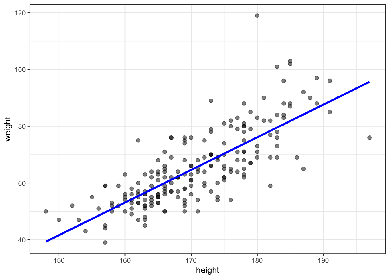

56.10 Observed Data, Fits, and Residuals

We observe data \((x_1, y_1), \ldots, (x_n, y_n)\). Note that we only observe \(X_i\) and \(Y_i\) from the generative model \(Y_i = \beta_1 + \beta_2 X_i + E_i\).

We calculate fitted values and observed residuals:

\[\hat{y}_i = \hat{\beta}_1 + \hat{\beta}_2 x_i\]

\[\hat{e}_i = y_i - \hat{y}_i\]

By construction, it is the case that \(\sum_{i=1}^n \hat{e}_i = 0\).

56.11 Proportion of Variation Explained

The proportion of variance explained by the fitted model is called \(R^2\) or \(r^2\). It is calculated by:

\[r^2 = \frac{s^2_{\hat{y}}}{s^2_{y}}\]