50 Bootstrap

50.1 Rationale

Suppose \(X_1, X_2, \ldots, X_n {\; \stackrel{\text{iid}}{\sim}\;}F\). If the edf \(\hat{F}_{{\boldsymbol{X}}}\) is an accurate approximation for the true cdf \(F\), then we can utilize \(\hat{F}_{{\boldsymbol{X}}}\) in place of \(F\) to nonparametrically characterize the sampling distribution of a statistic \(T({\boldsymbol{X}})\).

This allows for the sampling distribution of more general statistics to be considered, such as the median or a percentile, as well as more traditional statistics, such as the mean, when the underlying distribution is unknown.

When we encounter modeling fitting, the bootstrap may be very useful for characterizing the sampling distribution of complex statistics we calculate from fitted models.

50.2 Big Picture

We calculate \(T({\boldsymbol{x}})\) on the observed data, and we also form the edf, \(\hat{F}_{{\boldsymbol{x}}}\).

To approximate the sampling distribution of \(T({\boldsymbol{X}})\) we generate \(B\) random samples of \(n\) iid data points from \(\hat{F}_{{\boldsymbol{x}}}\) and calculate \(T({\boldsymbol{x}}^{*(b)})\) for each bootstrap sample \(b = 1, 2, \ldots, B\) where \({\boldsymbol{x}}^{*(b)} = (x_1^{*(b)}, x_2^{*(b)}, \ldots, x_n^{*(b)})^T\).

Sampling \(X_1^{*}, \ldots, X_n^{*} {\; \stackrel{\text{iid}}{\sim}\;}\hat{F}_{{\boldsymbol{x}}}\) is accomplished by sampling \(n\) times with replacement from the observed data \(x_1, x_2, \ldots, x_n\).

This means \(\Pr\left(X^{*} = x_j\right) = \frac{1}{n}\) for all \(j\).

50.3 Bootstrap Variance

For each bootstrap sample \({\boldsymbol{x}}^{*(b)} = (x_1^{*(b)}, x_2^{*(b)}, \ldots, x_n^{*(b)})^T\), calculate bootstrap statistic \(T({\boldsymbol{x}}^{*(b)})\).

Repeat this for \(b = 1, 2, \ldots, B\).

Estimate the sampling variance of \(T({\boldsymbol{x}})\) by

\[ \hat{{\operatorname{Var}}}(T({\boldsymbol{x}})) = \frac{1}{B} \sum_{b=1}^B \left(T\left({\boldsymbol{x}}^{*(b)}\right) - \frac{1}{B} \sum_{k=1}^B T\left({\boldsymbol{x}}^{*(k)}\right) \right)^2 \]

50.4 Caveat

Why haven’t we just been doing this the entire time?!

In All of Nonparametric Statistics, Larry Wasserman states:

There is a tendency to treat the bootstrap as a panacea for all problems. But the bootstrap requires regularity conditions to yield valid answers. It should not be applied blindly.

The bootstrap is easy to motivate, but it is quite tricky to implement outside of the very standard problems. It sometimes requires deeper knowledge of statistical theory than likelihood-based inference.

50.5 Bootstrap Sample

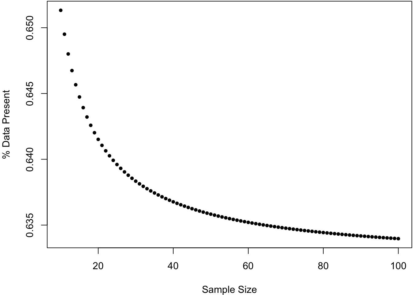
For a sample of size \(n\), what percentage of the data is present in any given bootstrap sample?

50.6 Bootstrap CIs

Suppose that \(\theta = T(F)\) and \(\hat{\theta} = T(\hat{F}_{{\boldsymbol{x}}})\).

We can use the bootstrap to generate data from \(\hat{F}_{{\boldsymbol{x}}}\).

For \(b = 1, 2, \ldots, B\), we draw \(x_1^{*(b)}, x_2^{*(b)}, \ldots, x_n^{*(b)}\) as iid realiztions from \(\hat{F}_{{\boldsymbol{x}}}\), and calculate \(\hat{\theta}^{*(b)} = T(\hat{F}_{{\boldsymbol{x}}^{*(b)}})\).

Let \(p^{*}_{\alpha}\) be the \(\alpha\) percentile of \(\left\{\hat{\theta}^{*(1)}, \hat{\theta}^{*(2)}, \ldots, \hat{\theta}^{*(B)}\right\}\).

Let’s discuss several ways of calculating confidence intervals for \(\theta = T(F)\).

50.7 Invoking the CLT

If we have evidence that the central limit theorem can be applied, we can form the \((1-\alpha)\) CI as:

\[ (\hat{\theta} - |z_{\alpha/2}| {\operatorname{se}}^*, \hat{\theta} + |z_{\alpha/2}| {\operatorname{se}}^*) \]

where \({\operatorname{se}}^*\) is the bootstrap standard error calculated as

\[ {\operatorname{se}}^{*} = \sqrt{\frac{1}{B} \sum_{b=1}^B \left(\hat{\theta}^{*(b)} - \frac{1}{B} \sum_{k=1}^B \hat{\theta}^{*(k)} \right)^2}. \]

 

Note that \({\operatorname{se}}^*\) serves as estimate of \({\operatorname{se}}(\hat{\theta})\).

Note that to get this confidence interval we need to justify that the following pivotal statistics are approximately Normal(0,1):

\[ \frac{\hat{\theta} - \theta}{{\operatorname{se}}(\hat{\theta})} \approx \frac{\hat{\theta} - \theta}{{\operatorname{se}}^*} \]

50.8 Percentile Interval

If a monotone function \(m(\cdot)\) exists so that \(m\left(\hat{\theta}\right) \sim \mbox{Normal}(m(\theta), b^2)\), then we can form the \((1-\alpha)\) CI as:

\[ \left(p^*_{\alpha/2}, p^*_{1-\alpha/2} \right) \]

where recall that in general \(p^{*}_{\alpha}\) is the \(\alpha\) percentile of bootstrap estimates \(\left\{\hat{\theta}^{*(1)}, \hat{\theta}^{*(2)}, \ldots, \hat{\theta}^{*(B)}\right\}\)

50.9 Pivotal Interval

Suppose we can calculate percentiles of \(\hat{\theta} - \theta\), say \(q_{\alpha}\). Note that the \(\alpha\) percentile of \(\hat{\theta}\) is \(q_\alpha + \theta\). The \(1-\alpha\) CI is

\[ (\hat{\theta}-q_{1-\alpha/2}, \hat{\theta}-q_{\alpha/2}) \]

which comes from:

\[ \begin{aligned} 1-\alpha & = \Pr(q_{\alpha/2} \leq \hat{\theta} - \theta \leq q_{1-\alpha/2}) \\ & = \Pr(-q_{1-\alpha/2} \leq \theta - \hat{\theta} \leq -q_{\alpha/2}) \\ & = \Pr(\hat{\theta}-q_{1-\alpha/2} \leq \theta \leq \hat{\theta}-q_{\alpha/2}) \\ \end{aligned} \]

Suppose the sampling distribution of \(\hat{\theta}^* - \hat{\theta}\) is an approximation for that of \(\hat{\theta} - \theta\).

If \(p^*_{\alpha}\) is the \(\alpha\) percentile of \(\hat{\theta}^*\) then, \(p^*_{\alpha} - \hat{\theta}\) is the \(\alpha\) percentile of \(\hat{\theta}^* - \hat{\theta}\).

Therefore, \(p^*_{\alpha} - \hat{\theta}\) is the bootstrap estimate of \(q_{\alpha}\). Plugging this into \((\hat{\theta}-q_{1-\alpha/2}, \hat{\theta}-q_{\alpha/2})\), we get the following \((1-\alpha)\) bootstrap CI:

\[ \left(2\hat{\theta}-p^*_{1-\alpha/2}, 2\hat{\theta}-p^*_{\alpha/2}\right). \]

50.10 Studentized Pivotal Interval

In the previous scenario, we needed to assume that the sampling distribution of \(\hat{\theta}^* - \hat{\theta}\) is an approximation for that of \(\hat{\theta} - \theta\). Sometimes this will not be the case and instead we can studentize this pivotal quantity. That is, the distribution of

\[ \frac{\hat{\theta} - \theta}{\hat{{\operatorname{se}}}\left(\hat{\theta}\right)} \]

is well-approximated by that of

\[ \frac{\hat{\theta}^* - \hat{\theta}}{\hat{{\operatorname{se}}}\left(\hat{\theta}^{*}\right)}. \]

Let \(z^{*}_{\alpha}\) be the \(\alpha\) percentile of

\[ \left\{ \frac{\hat{\theta}^{*(1)} - \hat{\theta}}{\hat{{\operatorname{se}}}\left(\hat{\theta}^{*(1)}\right)}, \ldots, \frac{\hat{\theta}^{*(B)} - \hat{\theta}}{\hat{{\operatorname{se}}}\left(\hat{\theta}^{*(B)}\right)} \right\}. \]

 

Then a \((1-\alpha)\) bootstrap CI is

\[ \left(\hat{\theta} - z^{*}_{1-\alpha/2} \hat{{\operatorname{se}}}\left(\hat{\theta}\right), \hat{\theta} - z^{*}_{\alpha/2} \hat{{\operatorname{se}}}\left(\hat{\theta}\right)\right). \]

 

Exercise: Why?

How do we obtain \(\hat{{\operatorname{se}}}\left(\hat{\theta}\right)\) and \(\hat{{\operatorname{se}}}\left(\hat{\theta}^{*(b)}\right)\)?

If we have an analytical formula for these, then \(\hat{{\operatorname{se}}}(\hat{\theta})\) is calculated from the original data and \(\hat{{\operatorname{se}}}(\hat{\theta}^{*(b)})\) from the bootstrap data sets. But we probably don’t since we’re using the bootstrap.

Instead, we can calculate:

\[ \hat{{\operatorname{se}}}\left(\hat{\theta}\right) = \sqrt{\frac{1}{B} \sum_{b=1}^B \left(\hat{\theta}^{*(b)} - \frac{1}{B} \sum_{k=1}^B \hat{\theta}^{*(k)} \right)^2}. \]

This is what we called \({\operatorname{se}}^*\) above. But what about \(\hat{{\operatorname{se}}}\left(\hat{\theta}^{*(b)}\right)\)?

To estimate \(\hat{{\operatorname{se}}}\left(\hat{\theta}^{*(b)}\right)\) we need to do a double bootstrap. For each bootstrap sample \(b\) we need to bootstrap that daat set another \(B\) times to calculate:

\[ \hat{{\operatorname{se}}}\left(\hat{\theta}^{*(b)}\right) = \sqrt{\frac{1}{B} \sum_{v=1}^B \left(\hat{\theta}^{*(b)*(v)} - \frac{1}{B} \sum_{k=1}^B \hat{\theta}^{*(b)*(k)} \right)^2} \]

where \(\hat{\theta}^{*(b)*(v)}\) is the statistic calculated from bootstrap sample \(v\) within bootstrap sample \(b\). This can be very computationally intensive, and it requires a large sample size \(n\).

50.11 Bootstrap Hypothesis Testing

As we have seen, hypothesis testing and confidence intervals are very related. For a simple null hypothesis, a bootstrap hypothesis test p-value can be calculated by finding the minimum \(\alpha\) for which the \((1-\alpha)\) CI does not contain the null hypothesis value. You showed this on your homework.

The general approach is to calculate a test statistic based on the observed data. Then the null distribution of this statistic is approximated by forming bootstrap test statistics under the scenario that the null hypothesis is true. This can often be accomplished because the \(\hat{\theta}\) estimated from the observed data is the population parameter from the bootstrap distribution.

50.12 Example: t-test

Suppose \(X_1, X_2, \ldots, X_m {\; \stackrel{\text{iid}}{\sim}\;}F_X\) and \(Y_1, Y_2, \ldots, Y_n {\; \stackrel{\text{iid}}{\sim}\;}F_Y\). We wish to test \(H_0: \mu(F_X) = \mu(F_Y)\) vs \(H_1: \mu(F_X) \not= \mu(F_Y)\). Suppose that we know \(\sigma^2(F_X) = \sigma^2(F_Y)\) (if not, it is straightforward to adjust the proecure below).

Our test statistic is

\[ t = \frac{\overline{x} - \overline{y}}{\sqrt{\left(\frac{1}{m} + \frac{1}{n}\right) s^2}} \]

where \(s^2\) is the pooled sample variance.

Note that the bootstrap distributions are such that \(\mu(\hat{F}_{X^{*}}) = \overline{x}\) and \(\mu(\hat{F}_{Y^{*}}) = \overline{y}\). Thus we want to center the bootstrap t-statistics about these known means.

Specifically, for a bootstrap data set \(x^{*} = (x_1^{*}, x_2^{*}, \ldots, x_m^{*})^T\) and \(y^{*} = (y_1^{*}, y_2^{*}, \ldots, y_n^{*})^T\), we form null t-statistic

\[ t^{*} = \frac{\overline{x}^{*} - \overline{y}^{*} - (\overline{x} - \overline{y})}{\sqrt{\left(\frac{1}{m} + \frac{1}{n}\right) s^{2*}}} \]

where again \(s^{2*}\) is the pooled sample variance.

In order to obtain a p-value, we calculate \(t^{*(b)}\) for \(b=1, 2, \ldots, B\) bootstrap data sets.

The p-value of \(t\) is then the proportion of bootstrap statistics as or more extreme than the observed statistic:

\[ \mbox{p-value}(t) = \frac{1}{B} \sum_{b=1}^{B} 1\left(|t^{*(b)}| \geq |t|\right). \]

50.13 Parametric Bootstrap

Suppose \(X_1, X_2, \ldots, X_n {\; \stackrel{\text{iid}}{\sim}\;}F_\theta\) for some parametric \(F_\theta\). We form estimate \(\hat{\theta}\), but we don’t have a known sampling distribution we can use to do inference with \(\hat{\theta}\).

The parametric bootstrap generates bootstrap data sets from \(F_{\hat{\theta}}\) rather than from the edf. It proceeds as we outlined above for these bootstrap data sets.

50.14 Example: Exponential Data

In the homework, you will be performing a bootstrap t-test of the mean and a bootstrap percentile CI of the median for the following Exponential(\(\lambda\)) data:

> set.seed(1111)
> pop.mean <- 2
> X <- matrix(rexp(1000*30, rate=1/pop.mean), nrow=1000, ncol=30)

Let’s construct a pivotal bootstrap CI of the median here instead.

> # population median 2*log(2)
> pop_med <- qexp(0.5, rate=1/pop.mean); pop_med
[1] 1.386294
> 
> obs_meds <- apply(X, 1, median)
> plot(density(obs_meds, adj=1.5), main=" "); abline(v=pop_med)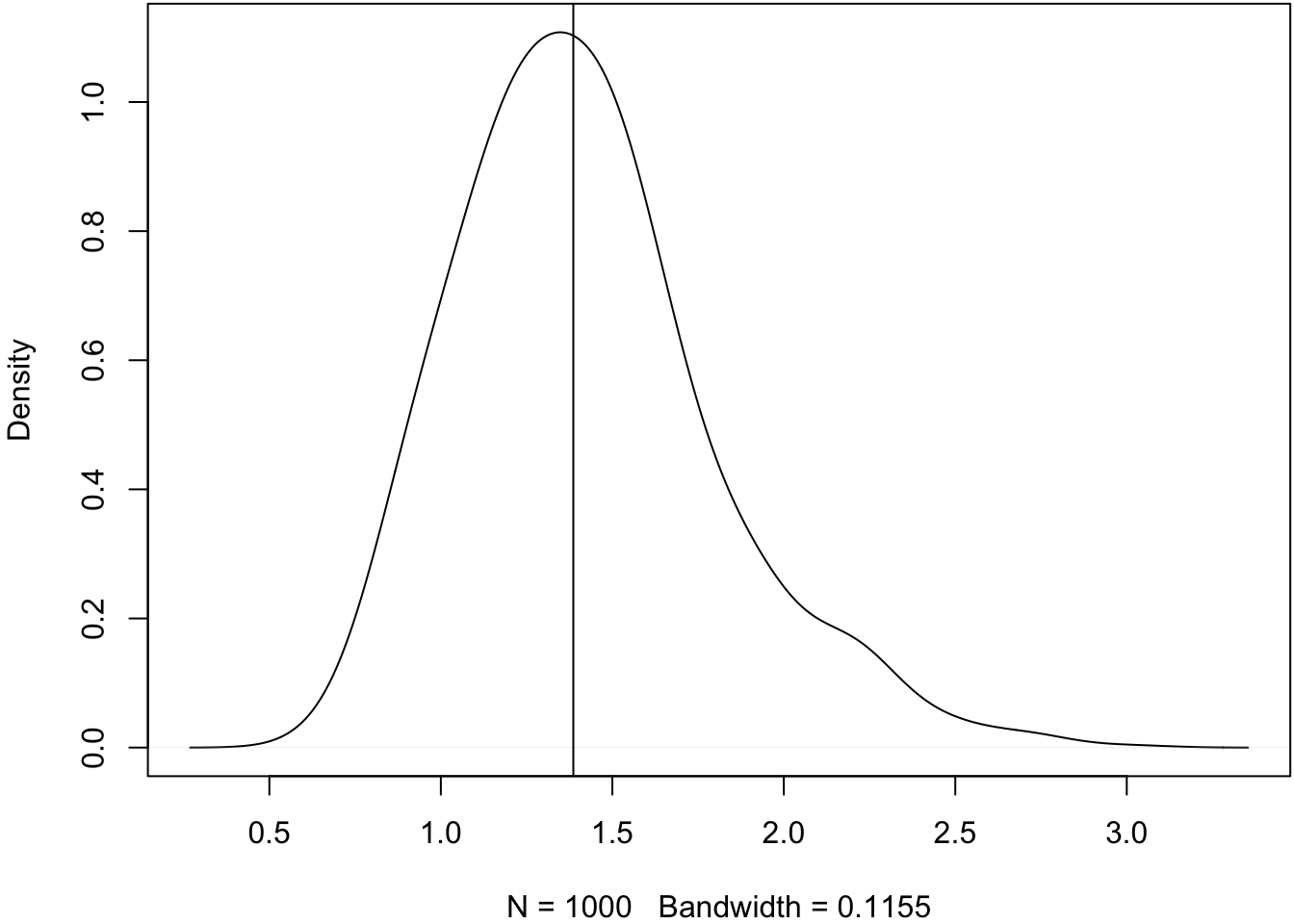

Some embarrassingly inefficient code to calculate bootstrap medians.

> B <- 1000
> boot_meds <- matrix(0, nrow=1000, ncol=B)
> 
> for(b in 1:B) {
+   idx <- sample(1:30, replace=TRUE)
+   boot_meds[,b] <- apply(X[,idx], 1, median)
+ }

Plot the bootstrap medians.

> plot(density(obs_meds, adj=1.5), main=" "); abline(v=pop_med)
> lines(density(as.vector(boot_meds[1:4,]), adj=1.5), col="red")
> lines(density(as.vector(boot_meds), adj=1.5), col="blue")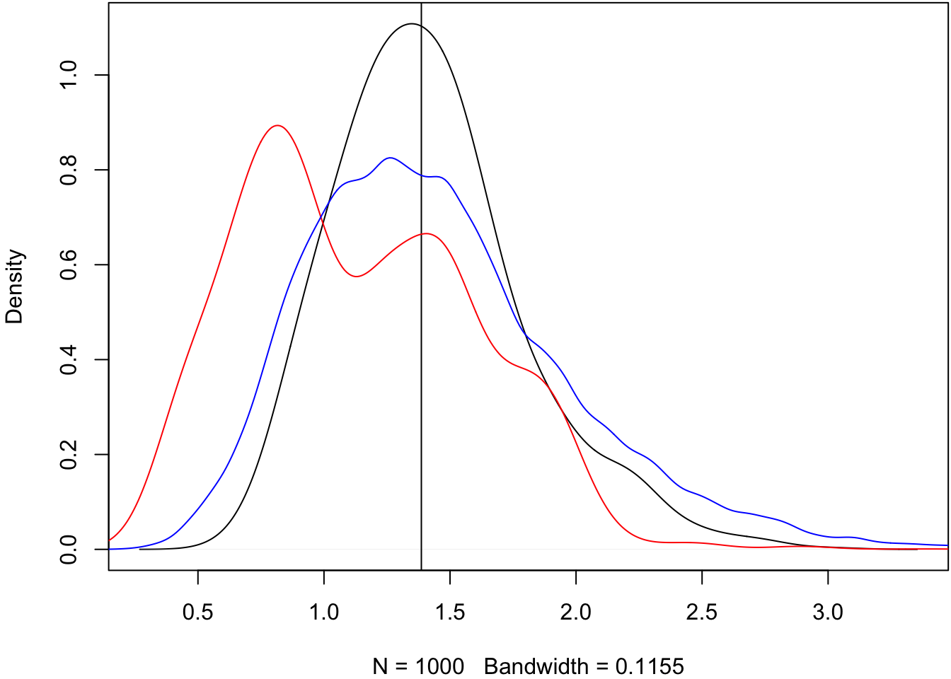

Compare sampling distribution of \(\hat{\theta}-\theta\) to \(\hat{\theta}^{*} - \hat{\theta}\).

> v <- obs_meds - pop_med
> w <- as.vector(boot_meds - obs_meds)
> qqplot(v, w, pch=20); abline(0,1)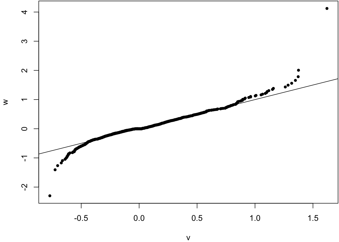

Does a 95% bootstrap pivotal interval provide coverage?

> ci_lower <- apply(boot_meds, 1, quantile, probs=0.975)
> ci_upper <- apply(boot_meds, 1, quantile, probs=0.025)
> 
> ci_lower <- 2*obs_meds - ci_lower
> ci_upper <- 2*obs_meds - ci_upper
> 
> ci_lower[1]; ci_upper[1]
[1] 0.8958224
[1] 2.113859
> 
> cover <- (pop_med >= ci_lower) & (pop_med <= ci_upper)
> mean(cover)
[1] 0.809
> 
> # :-(

Let’s check the bootstrap variances.

> sampling_var <- var(obs_meds)
> boot_var <- apply(boot_meds, 1, var)
> plot(density(boot_var, adj=1.5), main=" ")
> abline(v=sampling_var)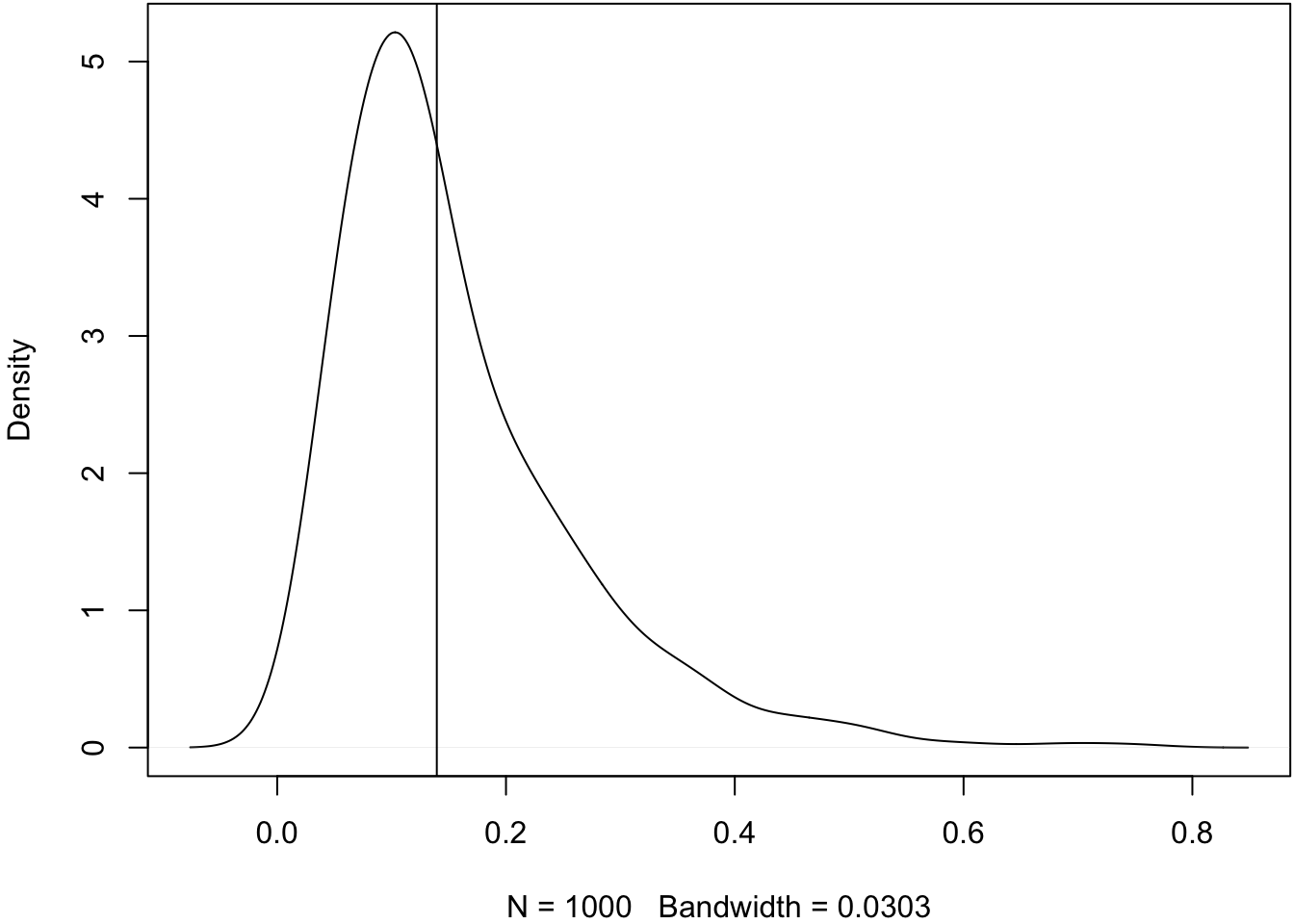

We repeated this simulation over a range of \(n\) and \(B\).

n	B	coverage	avg CI width
1e+02	1000	0.868	0.7805404
1e+02	2000	0.872	0.7882278
1e+02	4000	0.865	0.7852837
1e+02	8000	0.883	0.7817222
1e+03	1000	0.923	0.2465840
1e+03	2000	0.909	0.2477463
1e+03	4000	0.915	0.2475550
1e+03	8000	0.923	0.2458167
1e+04	1000	0.935	0.0781421
1e+04	2000	0.937	0.0784541
1e+04	4000	0.942	0.0784559
1e+04	8000	0.948	0.0785591
1e+05	1000	0.949	0.0246918
1e+05	2000	0.942	0.0246938