49 Empirical Distribution Functions
49.1 Definition
Suppose \(X_1, X_2, \ldots, X_n {\; \stackrel{\text{iid}}{\sim}\;}F\). The empirical distribution function (edf) – or empirical cumulative distribution function (ecdf) – is the distribution that puts probability \(1/n\) on each observed value \(X_i\).
Let \(1(X_i \leq y) = 1\) if \(X_i \leq y\) and \(1(X_i \leq y) = 0\) if \(X_i > y\).
\[ \mbox{Random variable: } \hat{F}_{{\boldsymbol{X}}}(y) = \frac{1}{n} \sum_{i=1}^{n} 1(X_i \leq y) \]
\[ \mbox{Observed variable: } \hat{F}_{{\boldsymbol{x}}}(y) = \frac{1}{n} \sum_{i=1}^{n} 1(x_i \leq y) \]
49.2 Example: Normal
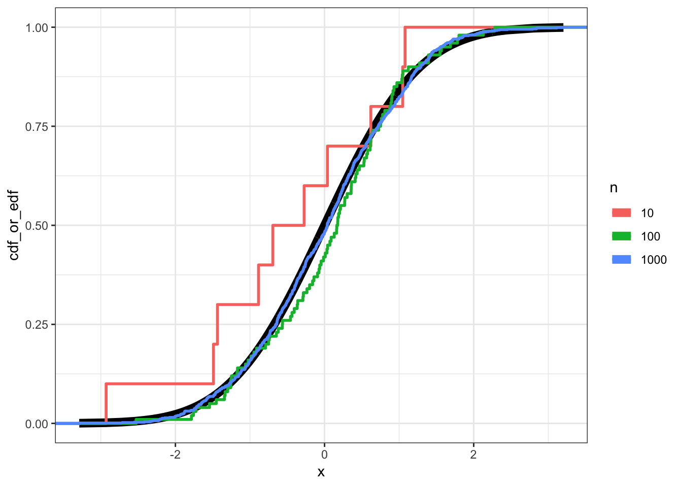
49.3 Pointwise Convergence
Under our assumptions, by the strong law of large numbers for each \(y \in \mathbb{R}\),
\[ \hat{F}_{{\boldsymbol{X}}}(y) \stackrel{\text{a.s.}}{\longrightarrow} F(y) \]
as \(n \rightarrow \infty\).
49.4 Glivenko-Cantelli Theorem
Under our assumptions, we can get a much stronger convergence result:
\[ \sup_{y \in \mathbb{R}} \left| \hat{F}_{{\boldsymbol{X}}}(y) - F(y) \right| \stackrel{\text{a.s.}}{\longrightarrow} 0 \]
as \(n \rightarrow \infty\). Here, “sup” is short for supremum, which is a mathematical generalization of maximum.
This result says that even the worst difference between the edf and the true cdf converges with probability 1 to zero.
49.5 Dvoretzky-Kiefer-Wolfowitz (DKW) Inequality
This result gives us an upper bound on how far off the edf is from the true cdf, which allows us to construct confidence bands about the edf.
\[ \Pr\left( \sup_{y \in \mathbb{R}} \left| \hat{F}_{{\boldsymbol{X}}}(y) - F(y) \right| > \epsilon \right) \leq 2 \exp{-2 n \epsilon^2} \]
As outlined in All of Nonparametric Statistics, setting
\[\epsilon_n = \sqrt{\frac{1}{2n} \log\left(\frac{2}{\alpha}\right)}\]
\[L(y) = \max\{\hat{F}_{{\boldsymbol{X}}}(y) - \epsilon_n, 0 \}\]
\[U(y) = \min\{\hat{F}_{{\boldsymbol{X}}}(y) + \epsilon_n, 1 \}\]
guarantees that \(\Pr(L(y) \leq F(y) \leq U(y) \mbox{ for all } y) \geq 1-\alpha\).
49.6 Statistical Functionals
A statistical functional \(T(F)\) is any function of \(F\). Examples:
- \(\mu(F) = \int x dF(x)\)
- \(\sigma^2(F) = \int (x-\mu(F))^2 dF(x)\)
- \(\text{median}(F) = F^{-1}(1/2)\)
A linear statistical functional is such that \(T(F) = \int a(x) dF(x)\).
49.7 Plug-In Estimator
A plug-in estimator of \(T(F)\) based on the edf is \(T(\hat{F}_{{\boldsymbol{X}}})\). Examples:
\(\hat{\mu} = \mu(\hat{F}_{{\boldsymbol{X}}}) = \int x \hat{F}_{{\boldsymbol{X}}}(x) = \frac{1}{n} \sum_{i=1}^n X_i\)
\(\hat{\sigma}^2 = \sigma^2(\hat{F}_{{\boldsymbol{X}}}) = \int (x-\hat{\mu})^2 \hat{F}_{{\boldsymbol{X}}}(x) = \frac{1}{n} \sum_{i=1}^n (X_i - \hat{\mu})^2\)
\(\text{median}(\hat{F}_{{\boldsymbol{X}}}) = \hat{F}_{{\boldsymbol{X}}}^{-1}(1/2)\)
49.8 EDF Standard Error
Suppose that \(T(F) = \int a(x) dF(x)\) is a linear functional. Then:
\[ \begin{aligned} \ & {\operatorname{Var}}(T(\hat{F}_{{\boldsymbol{X}}})) = \frac{1}{n^2} \sum_{i=1}^n {\operatorname{Var}}(a(X_i)) = \frac{{\operatorname{Var}}_F(a(X))}{n} \\ \ & {\operatorname{se}}(T(\hat{F}_{{\boldsymbol{X}}})) = \sqrt{\frac{{\operatorname{Var}}_F(a(X))}{n}} \\ \ & \hat{{\operatorname{se}}}(T(\hat{F}_{{\boldsymbol{X}}})) = \sqrt{\frac{{\operatorname{Var}}_{\hat{F}_{{\boldsymbol{X}}}}(a(X))}{n}} \end{aligned} \]
Note that
\[ {\operatorname{Var}}_F(a(X)) = \int (a(x) - T(F))^2 dF(x) \] because \(T(F) = \int a(x) dF(x) = {\operatorname{E}}_F[a(X)]\). Likewise,
\[ {\operatorname{Var}}_{\hat{F}_{{\boldsymbol{X}}}}(a(X)) = \frac{1}{n} \sum_{i=1}^n (a(X_i) - T(\hat{F}_{{\boldsymbol{X}}}))^2 \]
where \(T(\hat{F}_{{\boldsymbol{X}}}) = \frac{1}{n} \sum_{i=1}^n a(X_i)\).
49.9 EDF CLT
Suppose that \({\operatorname{Var}}_F(a(X)) < \infty\). Then we have the following convergences as \(n \rightarrow \infty\):
\[ \frac{{\operatorname{Var}}_{\hat{F}_{{\boldsymbol{X}}}}(a(X))}{{\operatorname{Var}}_{F}(a(X))} \stackrel{P}{\longrightarrow} 1 \mbox{ , } \frac{\hat{{\operatorname{se}}}(T(\hat{F}_{{\boldsymbol{X}}}))}{{\operatorname{se}}(T(\hat{F}_{{\boldsymbol{X}}}))} \stackrel{P}{\longrightarrow} 1 \]
\[ \frac{T(F) - T(\hat{F}_{{\boldsymbol{X}}})}{\hat{{\operatorname{se}}}(T(\hat{F}_{{\boldsymbol{X}}}))} \stackrel{D}{\longrightarrow} \mbox{Normal}(0,1) \]
The estimators are very easy to calculate on real data, so this a powerful set of results.