70 High-Dimensional Data and Inference
70.1 Definition
High-dimesional inference is the scenario where we perform inference simultaneously on “many” paramaters.
“Many” can be as few as three parameters (which is where things start to get interesting), but in modern applications this is typically on the order of thousands to billions of paramaters.
High-dimesional data is a data set where the number of variables measured is many.
Large sample size data is a data set where few variables are measured, but many observations are measured.
Big data is a data set where there are so many data points that it cannot be managed straightforwardly in memory, but must rather be stored and accessed elsewhere. Big data can be high-dimensional, large sample size, or both.
We will abbreviate high-dimensional with HD.
70.2 Examples
In all of these examples, many measurements are taken and the goal is often to perform inference on many paramaters simultaneously.
- Spatial epidemiology
- Environmental monitoring
- Internet user behavior
- Genomic profiling
- Neuroscience imaging
- Financial time series
70.3 HD Gene Expression Data
> knitr::include_graphics("./images/rna_sequencing.png")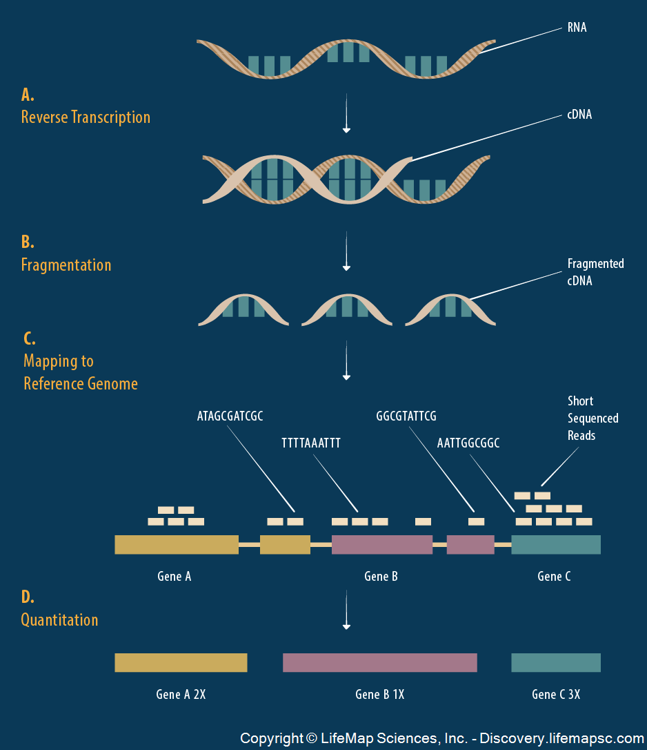
It’s possible to measure the level of gene expression – how much mRNA is being transcribed – from thousands of cell simultaneously in a single biological sample.
Typically, gene expression is measured over varying biological conditions, and the goal is to perform inference on the relationship between expression and the varying conditions.
This results in thousands of simultaneous inferences.
The typical sizes of these data sets are 1000 to 50,000 genes and 10 to 1000 observations.
The gene expression values are typically modeled as approximately Normal or overdispersed Poisson.
There is usually shared signal among the genes, and there are often unobserved latent variables.
\[ \begin{array}{rc} & {\boldsymbol{Y}}_{m \times n} \\ & \text{observations} \\ \text{genes} & \begin{bmatrix} y_{11} & y_{12} & \cdots & y_{1n} \\ y_{21} & y_{22} & \cdots & y_{2n} \\ & & & \\ \vdots & \vdots & \ddots & \vdots \\ & & & \\ y_{m1} & y_{m2} & \cdots & y_{mn} \end{bmatrix} \\ & \\ & {\boldsymbol{X}}_{d \times n} \ \text{study design} \\ & \begin{bmatrix} x_{11} & x_{12} & \cdots & x_{1n} \\ \vdots & \vdots & \ddots & \vdots \\ x_{d1} & x_{d2} & \cdots & x_{dn} \end{bmatrix} \end{array} \]
The \({\boldsymbol{Y}}\) matrix contains gene expression measurements for \(m\) genes (rows) by \(n\) observations (columns). The values \(y_{ij}\) are either in \(\mathbb{R}\) or \(\mathbb{Z}^{+} = \{0, 1, 2, \ldots \}\).
The \({\boldsymbol{X}}\) matrix contains the study design of \(d\) explanatory variables (rows) by the \(n\) observations (columns).
Note that \(m \gg n \gg d\).
70.4 Many Responses Model
Gene expression is an example of what I call the many responses model.
We’re interested in performing simultaneous inference on \(d\) paramaters for each of \(m\) models such as:
\[ \begin{aligned} & {\boldsymbol{Y}}_{1} = {\boldsymbol{\beta}}_1 {\boldsymbol{X}}+ {\boldsymbol{E}}_1 \\ & {\boldsymbol{Y}}_{2} = {\boldsymbol{\beta}}_2 {\boldsymbol{X}}+ {\boldsymbol{E}}_2 \\ & \vdots \\ & {\boldsymbol{Y}}_{m} = {\boldsymbol{\beta}}_m {\boldsymbol{X}}+ {\boldsymbol{E}}_m \\ \end{aligned} \]
For example, \({\boldsymbol{Y}}_{1} = {\boldsymbol{\beta}}_1 {\boldsymbol{X}}+ {\boldsymbol{E}}_1\) is vector notation of (in terms of observations \(j\)):
\[ \left\{ Y_{1j} = \beta_{11} X_{1j} + \beta_{12} X_{2j} + \cdots + \beta_{1d} X_{dj} + E_{1j} \right\}_{j=1}^n \]
We have made two changes from last week:
- We have transposed \({\boldsymbol{X}}\) and \({\boldsymbol{\beta}}\).
- We have changed the number of explanatory variables from \(p\) to \(d\).
Let \({\boldsymbol{B}}_{m \times d}\) be the matrix of parameters \((\beta_{ik})\) relating the \(m\) response variables to the \(d\) explanatory variables. The full HD model is
\[ \begin{array}{cccccc} {\boldsymbol{Y}}_{m \times n} & = & {\boldsymbol{B}}_{m \times d} & {\boldsymbol{X}}_{d \times n} & + & {\boldsymbol{E}}_{m \times n} \\ \begin{bmatrix} & & \\ & & \\ & & \\ Y_{i1} & \cdots & Y_{in}\\ & & \\ & & \\ & & \\ \end{bmatrix} & = & \begin{bmatrix} & \\ & \\ & \\ \beta_{i1} & \beta_{id} \\ & \\ & \\ & \\ \end{bmatrix} & \begin{bmatrix} X_{11} & \cdots & X_{1n} \\ X_{d1} & \cdots & X_{dn} \\ \end{bmatrix} & + & \begin{bmatrix} & & \\ & & \\ & & \\ E_{i1} & \cdots & E_{in} \\ & & \\ & & \\ & & \\ \end{bmatrix} \end{array} \]
Note that if we make OLS assumptions, then we can calculate:
\[ \hat{{\boldsymbol{B}}}^{\text{OLS}} = {\boldsymbol{Y}}{\boldsymbol{X}}^T ({\boldsymbol{X}}{\boldsymbol{X}}^T)^{-1} \]
\[ \hat{{\boldsymbol{Y}}} = \hat{{\boldsymbol{B}}} {\boldsymbol{X}}= {\boldsymbol{Y}}{\boldsymbol{X}}^T ({\boldsymbol{X}}{\boldsymbol{X}}^T)^{-1} {\boldsymbol{X}}\]
so here the projection matrix is \({\boldsymbol{P}}= {\boldsymbol{X}}^T ({\boldsymbol{X}}{\boldsymbol{X}}^T)^{-1} {\boldsymbol{X}}\) and acts from the RHS, \(\hat{{\boldsymbol{Y}}} = {\boldsymbol{Y}}{\boldsymbol{P}}\).
We will see this week and next that \(\hat{{\boldsymbol{B}}}^{\text{OLS}}\) has nontrivial drawbacks. Thefore, we will be exploring other ways of estimating \({\boldsymbol{B}}\).
We of course aren’t limited to OLS models. We could consider the many response GLM:
\[ g\left({\operatorname{E}}\left[ \left. {\boldsymbol{Y}}_{m \times n} \right| {\boldsymbol{X}}\right]\right) = {\boldsymbol{B}}_{m \times d} {\boldsymbol{X}}_{d \times n} \]
and we could even replace \({\boldsymbol{B}}_{m \times d} {\boldsymbol{X}}_{d \times n}\) with \(d\) smoothers for each of the \(m\) response variable.
70.5 HD SNP Data
> knitr::include_graphics("./images/snp_dna.png")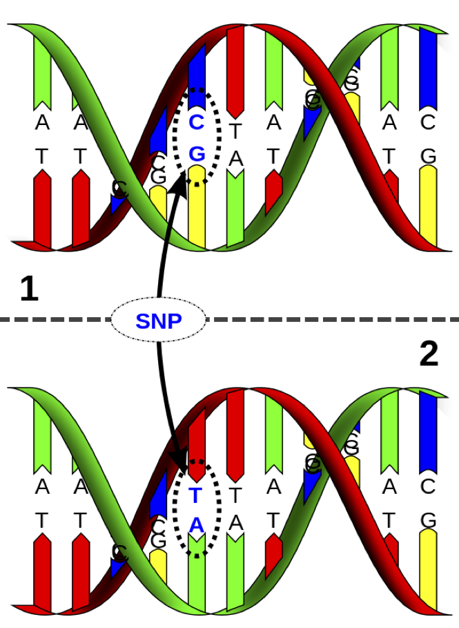
It is possible to measure single nucleotide polymorphisms at millions of locations across the genome.
The base (A, C, G, or T) is measured from one of the strands.
For example, on the figure to the left, the individual is heterozygous CT at this SNP location.
\[ \begin{array}{rc} & {\boldsymbol{X}}_{m \times n} \\ & \text{individuals} \\ \text{SNPs} & \begin{bmatrix} x_{11} & x_{12} & \cdots & x_{1n} \\ x_{21} & x_{22} & \cdots & x_{2n} \\ & & & \\ \vdots & \vdots & \ddots & \vdots \\ & & & \\ x_{m1} & x_{m2} & \cdots & x_{mn} \end{bmatrix} \\ & \\ & {\boldsymbol{y}}_{1 \times n} \ \text{trait} \\ & \begin{bmatrix} y_{11} & y_{12} & \cdots & y_{1n} \end{bmatrix} \end{array} \]
The \({\boldsymbol{X}}\) matrix contains SNP genotypes for \(m\) SNPs (rows) by \(n\) individuals (columns). The values \(x_{ij} \in \{0, 1, 2\}\) are conversions of genotypes (e.g., CC, CT, TT) to counts of one of the alleles.
The \({\boldsymbol{y}}\) vector contains the trait values of the \(n\) individuals.
Note that \(m \gg n\).
70.6 Many Regressors Model
The SNP-trait model is an example of what I call the many regressors model. A single model is fit of a response variable on many regressors (i.e., explanatory variables) simultaneously.
This involves simultaneously inferring \(m\) paramaters \({\boldsymbol{\beta}}= (\beta_1, \beta_2, \ldots, \beta_m)\) in models such as:
\[ {\boldsymbol{Y}}= \alpha \boldsymbol{1} + {\boldsymbol{\beta}}{\boldsymbol{X}}+ {\boldsymbol{E}}\]
which is an \(n\)-vector with component \(j\) being:
\[ Y_j = \alpha + \sum_{i=1}^m \beta_i X_{ij} + E_{j} \]
As with the many responses model, we do not need to limit the model to the OLS type where the response variable is approximately Normal distributed. Instead we can consider more general models such as
\[ g\left({\operatorname{E}}\left[ \left. {\boldsymbol{Y}}\right| {\boldsymbol{X}}\right]\right) = \alpha \boldsymbol{1} + {\boldsymbol{\beta}}{\boldsymbol{X}}\]
for some link function \(g(\cdot)\).
70.7 Goals
In both types of models we are interested in:
- Forming point estimates
- Testing statistical hypothesis
- Calculating posterior distributions
- Leveraging the HD data to increase our power and accuracy
Sometimes we are also interested in confidence intervals in high dimensions, but this is less common.
70.8 Challenges
Here are several of the new challenges we face when analyzing high-dimensional data:
- Standard estimation methods may be suboptimal in high dimensions
- New measures of significance are needed
- There may be dependence and latent variables among the high-dimensional variables
- The fact that \(m \gg n\) poses challenges, especially in the many regressors model
HD data provide new challenges, but they also provide opportunities to model variation in the data in ways not possible for low-dimensional data.