73 Multiple Testing
73.1 Motivating Example
Hedenfalk et al. (2001) NEJM measured gene expression in three different breast cancer tumor types. In your homework, you have analyzed these data and have specifically compared BRCA1 mutation positive tumors to BRCA2 mutation positive tumors.
The qvalue package has the p-values when testing for a difference in population means between these two groups (called “differential expression”). There are 3170 genes tested, resulting in 3170 p-values.
Note that this analysis is a version of the many responses model.
> library(qvalue)
> data(hedenfalk); df <- data.frame(p=hedenfalk$p)
> ggplot(df, aes(x = p)) +
+          ggtitle("p-value density histogram") +
+          geom_histogram(aes_string(y = '..density..'), colour = "black",
+                         fill = "white", binwidth = 0.04, center=0.02)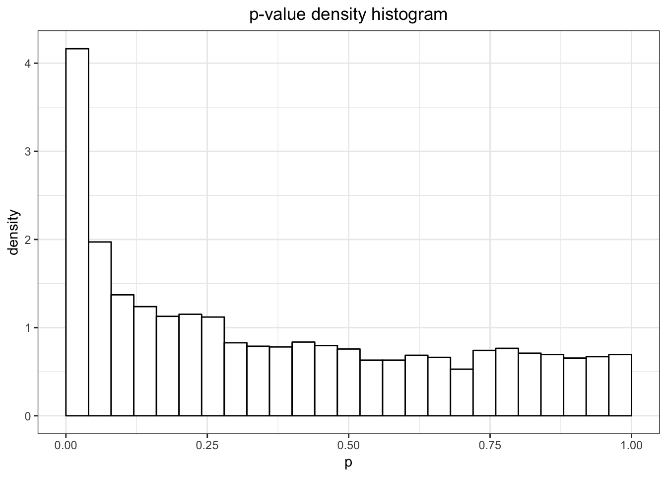
73.2 Challenges
- Traditional p-value thresholds such as 0.01 or 0.05 may result in too many false positives. For example, in the above example, a 0.05 threshold could result in 158 false positives.
- A careful balance of true positives and false positives must be achieved in a manner that is scientifically interpretable.
- There is information in the joint distribution of the p-values that can be leveraged.
- Dependent p-values may make this type of analysis especially difficult (next week’s topic).
> qobj <- qvalue(hedenfalk$p)
> hist(qobj)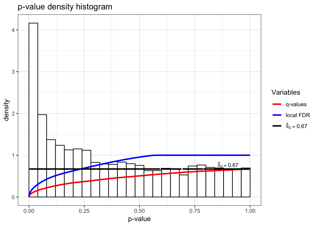
73.3 Outcomes
Possible outcomes from \(m\) hypothesis tests based on applying a significance threshold \(0 < t \leq 1\) to their corresponding p-values.
| Not Significant | Significant | Total | |
|---|---|---|---|
| Null True | \(U\) | \(V\) | \(m_0\) |
| Alternative True | \(T\) | \(S\) | \(m_1\) |
| Total | \(W\) | \(R\) | \(m\) |
73.4 Error Rates
Suppose we are testing \(m\) hypotheses based on p-values \(p_1, p_2, \ldots, p_m\).
Multiple hypothesis testing is the process of deciding which of these p-values should be called statistically significant.
This requires formulating and estimating a compound error rate that quantifies the quality of the decision.
73.5 Bonferroni Correction
The family-wise error rate is the probability of any false positive occurring among all tests called significant. The Bonferroni correction is a result that shows that utilizing a p-value threshold of \(\alpha/m\) results in FWER \(\leq \alpha\). Specifically,
\[ \begin{aligned} \text{FWER} & \leq \Pr(\cup \{P_i \leq \alpha/m\}) \\ & \leq \sum_{i=1}^m \Pr(P_i \leq \alpha/m) = \sum_{i=1}^m \alpha/m = \alpha \end{aligned} \]
where the above probability calculations are done under the assumption that all \(H_0\) are true.
73.6 False Discovery Rate
The false discovery rate (FDR) measures the proportion of Type I errors — or “false discoveries” — among all hypothesis tests called statistically significant. It is defined as
\[ {{\rm FDR}}= {\operatorname{E}}\left[ \frac{V}{R \vee 1} \right] = {\operatorname{E}}\left[ \left. \frac{V}{R} \right| R>0 \right] \Pr(R>0). \]
This is less conservative than the FWER and it offers a clearer balance between true positives and false positives.
There are two other false discovery rate definitions, where the main difference is in how the \(R=0\) event is handled. These quantities are called the positive false discovery rate (pFDR) and the marginal false discovery rate (mFDR), defined as follows:
\[ {{\rm pFDR}}= {\operatorname{E}}\left[ \left. \frac{V}{R} \right| R>0 \right], \]
\[ {{\rm mFDR}}= \frac{{\operatorname{E}}\left[ V \right]}{{\operatorname{E}}\left[ R \right]}. \]
Note that \({{\rm pFDR}}= {{\rm mFDR}}= 1\) whenever all null hypotheses are true, whereas FDR can always be made arbitrarily small because of the extra term \(\Pr(R > 0)\).
73.7 Point Estimate
Let \({{\rm FDR}}(t)\) denote the FDR when calling null hypotheses significant whenever \(p_i \leq t\), for \(i = 1, 2, \ldots, m\). For \(0 < t \leq 1\), we define the following random variables:
\[ \begin{aligned} V(t) & = \#\{\mbox{true null } p_i: p_i \leq t \} \\ R(t) & = \#\{p_i: p_i \leq t\} \end{aligned} \] In terms of these, we have
\[ {{\rm FDR}}(t) = {\operatorname{E}}\left[ \frac{V(t)}{R(t) \vee 1} \right]. \]
For fixed \(t\), the following defines a family of conservatively biased point estimates of \({{\rm FDR}}(t)\):
\[ \hat{{{\rm FDR}}}(t) = \frac{\hat{m}_0(\lambda) \cdot t}{[R(t) \vee 1]}. \]
The term \(\hat{m}_0({\lambda})\) is an estimate of \(m_0\), the number of true null hypotheses. This estimate depends on the tuning parameter \({\lambda}\), and it is defined as
\[ \hat{m}_0({\lambda}) = \frac{m - R({\lambda})}{(1-{\lambda})}. \]
Sometimes instead of \(m_0\), the quantity
\[ \pi_0 = \frac{m_0}{m} \]
is estimated, where simply
\[ \hat{\pi}_0({\lambda}) = \frac{\hat{m}_0({\lambda})}{m} = \frac{m - R({\lambda})}{m(1-{\lambda})}. \]
It can be shown that \({\operatorname{E}}[\hat{m}_0({\lambda})] \geq m_0\) when the p-values corresponding to the true null hypotheses are Uniform(0,1) distributed (or stochastically greater).
There is an inherent bias/variance trade-off in the choice of \({\lambda}\). In most cases, when \({\lambda}\) gets smaller, the bias of \(\hat{m}_0({\lambda})\) gets larger, but the variance gets smaller.
Therefore, \({\lambda}\) can be chosen to try to balance this trade-off.
73.8 Adaptive Threshold
If we desire a FDR level of \(\alpha\), it is tempting to use the p-value threshold
\[ t^*_\alpha = \max \left\{ t: \hat{{{\rm FDR}}}(t) \leq \alpha \right\} \]
which identifies the largest estimated FDR less than or equal to \(\alpha\).
73.9 Conservative Properties
When the p-value corresponding to true null hypothesis are distributed iid Uniform(0,1), then we have the following two conservative properties.
\[ \begin{aligned} & {\operatorname{E}}\left[ \hat{{{\rm FDR}}}(t) \right] \geq {{\rm FDR}}(t) \\ & {\operatorname{E}}\left[ \hat{{{\rm FDR}}}(t^*_\alpha) \right] \leq \alpha \end{aligned} \]
73.10 Q-Values
In single hypothesis testing, it is common to report the p-value as a measure of significance. The q-value is the FDR based measure of significance that can be calculated simultaneously for multiple hypothesis tests.
The p-value is constructed so that a threshold of \(\alpha\) results in a Type I error rate \(\leq \alpha\). Likewise, the q-value is constructed so that a threshold of \(\alpha\) results in a FDR \(\leq \alpha\).
Initially it seems that the q-value should capture the FDR incurred when the significance threshold is set at the p-value itself, \({{\rm FDR}}(p_i)\). However, unlike Type I error rates, the FDR is not necessarily strictly increasing with an increasing significance threshold.
To accommodate this property, the q-value is defined to be the minimum FDR (or pFDR) at which the test is called significant:
\[ {\operatorname{q}}{\rm\mbox{-}value}(p_i) = \min_{t \geq p_i} {{\rm FDR}}(t) \]
or
\[ {\operatorname{q}}{\rm\mbox{-}value}(p_i) = \min_{t \geq p_i} {{\rm pFDR}}(t). \]
To estimate this in practice, a simple plug-in estimate is formed, for example:
\[ \hat{{\operatorname{q}}}{\rm\mbox{-}value}(p_i) = \min_{t \geq p_i} \hat{{{\rm FDR}}}(t). \]
Various theoretical properties have been shown for these estimates under certain conditions, notably that the estimated q-values of the entire set of tests are simultaneously conservative as the number of hypothesis tests grows large.
> plot(qobj)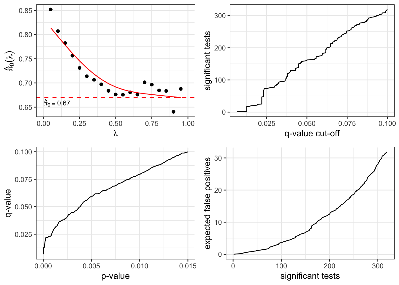
73.11 Bayesian Mixture Model
Let’s return to the Bayesian classification set up from earlier. Suppose that
- \(H_i =\) 0 or 1 according to whether the \(i\)th null hypothesis is true or not
- \(H_i {\; \stackrel{\text{iid}}{\sim}\;}\mbox{Bernoulli}(1-\pi_0)\) so that \(\Pr(H_i=0)=\pi_0\) and \(\Pr(H_i=1)=1-\pi_0\)
- \(P_i | H_i {\; \stackrel{\text{iid}}{\sim}\;}(1-H_i) \cdot F_0 + H_i \cdot F_1\), where \(F_0\) is the null distribution and \(F_1\) is the alternative distribution
73.12 Bayesian-Frequentist Connection
Under these assumptions, it has been shown that
\[ \begin{aligned} {{\rm pFDR}}(t) & = {\operatorname{E}}\left[ \left. \frac{V(t)}{R(t)} \right| R(t) > 0 \right] \\ \ & = \Pr(H_i = 0 | P_i \leq t) \end{aligned} \]
where \(\Pr(H_i = 0 | P_i \leq t)\) is the same for each \(i\) because of the iid assumptions.
Under these modeling assumptions, it follows that
\[ \mbox{q-value}(p_i) = \min_{t \geq p_i} \Pr(H_i = 0 | P_i \leq t) \]
which is a Bayesian analogue of the p-value — or rather a “Bayesian posterior Type I error rate”.
73.13 Local FDR
In this scenario, it also follows that
\[ {{\rm pFDR}}(t) = \int \Pr(H_i = 0 | P_i = p_i) dF(p_i | p_i \leq t) \]
where \(F = \pi_0 F_0 + (1-\pi_0) F_1\).
This connects the pFDR to the posterior error probability
\[\Pr(H_i = 0 | P_i = p_i)\]
making this latter quantity sometimes interpreted as a local false discovery rate.
> hist(qobj)