72 Shrinkage and Empirical Bayes

72.1 Estimating Several Means

Let’s start with the simplest many responses model where there is only an interncept and only one observation per variable. This means that \(n=1\) and \(d=1\) where \({\boldsymbol{X}}= 1\).

This model can be written as \(Y_i \sim \mbox{Normal}(\beta_i, 1)\) for the \(i=1, 2, \ldots, m\) response variables. Suppose also that \(Y_1, Y_2, \ldots, Y_m\) are jointly independent.

Let’s assume that \(\beta_1, \beta_2, \ldots, \beta_m\) are fixed, nonrandom parameters.

72.2 Usual MLE

The usual estimates of \(\beta_i\) are to set

\[ \hat{\beta}_i^{\text{MLE}} = {\boldsymbol{Y}}_i. \]

This is also the OLS solution.

72.3 Loss Function

Suppose we are interested in the simultaneous loss function

\[ L({\boldsymbol{\beta}}, \hat{{\boldsymbol{\beta}}}) = \sum_{i=1} (\beta_i - \hat{\beta}_i)^2 \]

with risk \(R({\boldsymbol{\beta}}, \hat{{\boldsymbol{\beta}}}) = {\operatorname{E}}[L({\boldsymbol{\beta}}, \hat{{\boldsymbol{\beta}}})]\).

72.4 Stein’s Paradox

Consider the following James-Stein estimator:

\[ \hat{\beta}_i^{\text{JS}} = \left(1 - \frac{m-2}{\sum_{k=1}^m Y_k^2} \right) Y_i. \]

In a shocking result called Stein’s paradox, it was shown that when \(m \geq 3\) then

\[ R\left({\boldsymbol{\beta}}, \hat{{\boldsymbol{\beta}}}^{\text{JS}}\right) < R\left({\boldsymbol{\beta}}, \hat{{\boldsymbol{\beta}}}^{\text{MLE}}\right). \]

This means that the usual MLE is dominated by this JS estimator for any, even nonrandom, configuration of \(\beta_1, \beta_2, \ldots, \beta_m\)!

What is going on?

Let’s first take a linear regression point of view to better understand this paradox.

Then we will return to the empirical Bayes example from earlier.

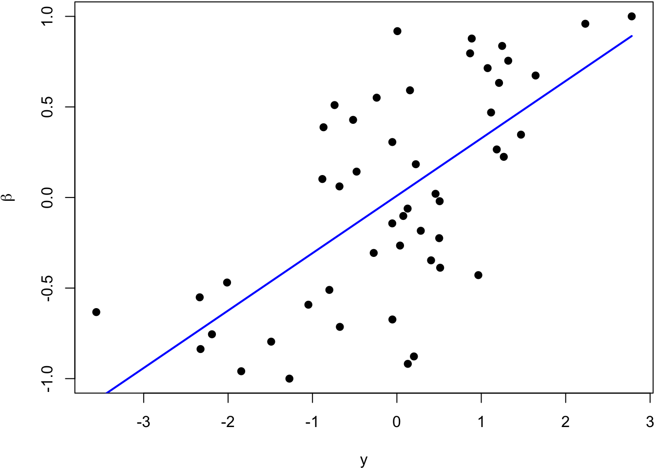
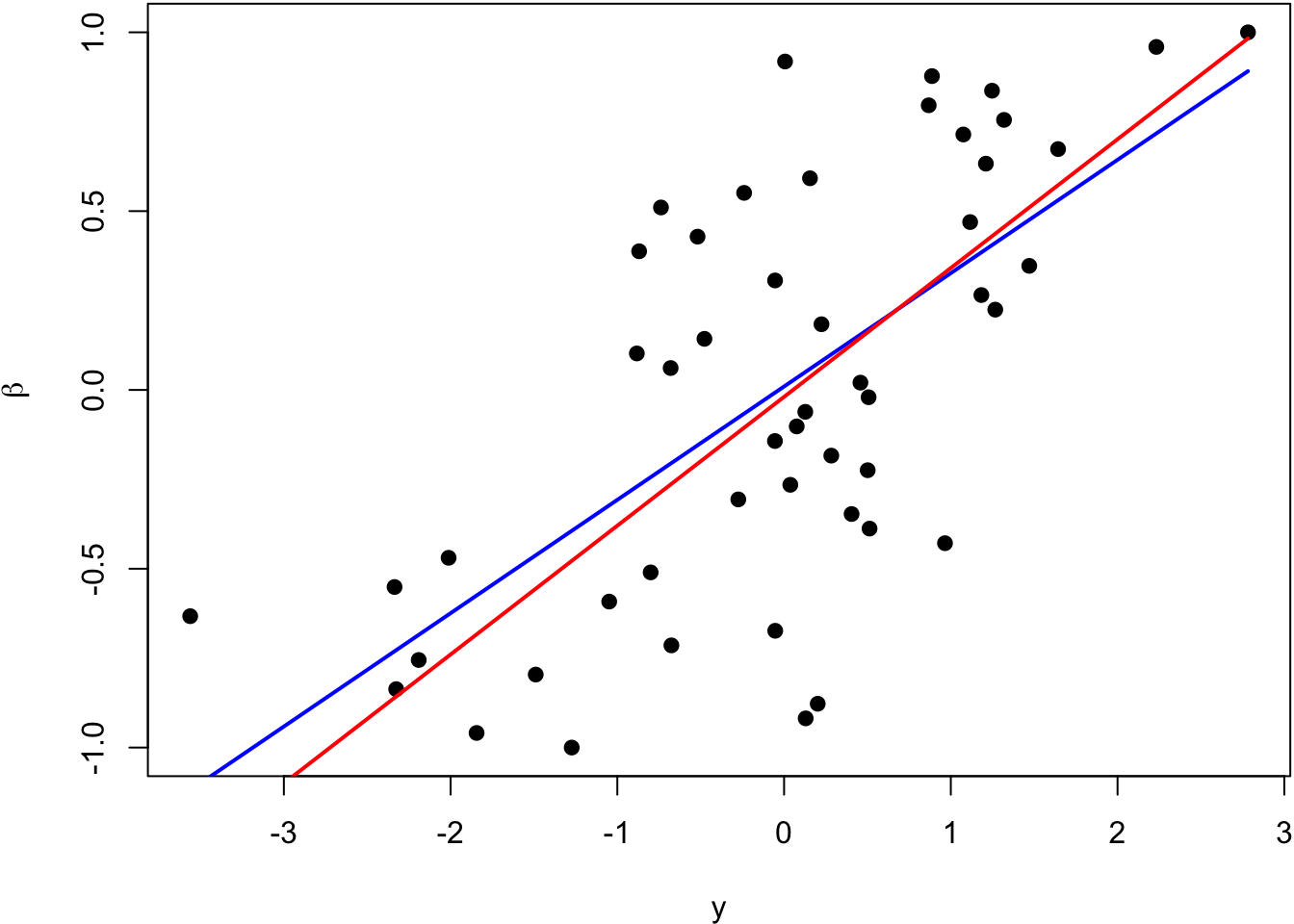
> beta <- seq(-1, 1, length.out=50)
> y <- beta + rnorm(length(beta))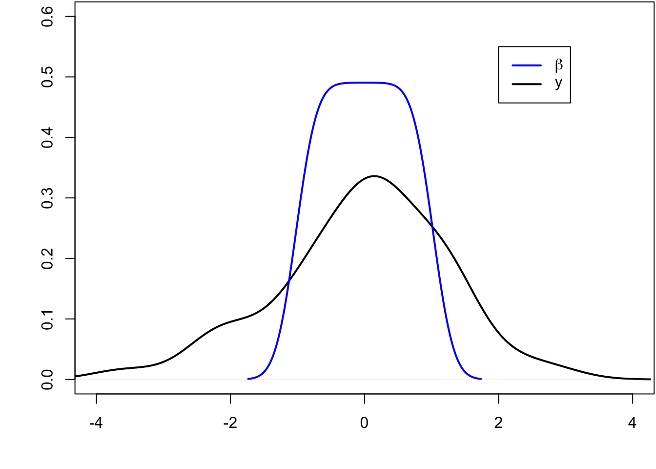

The blue line is the least squares regression line.

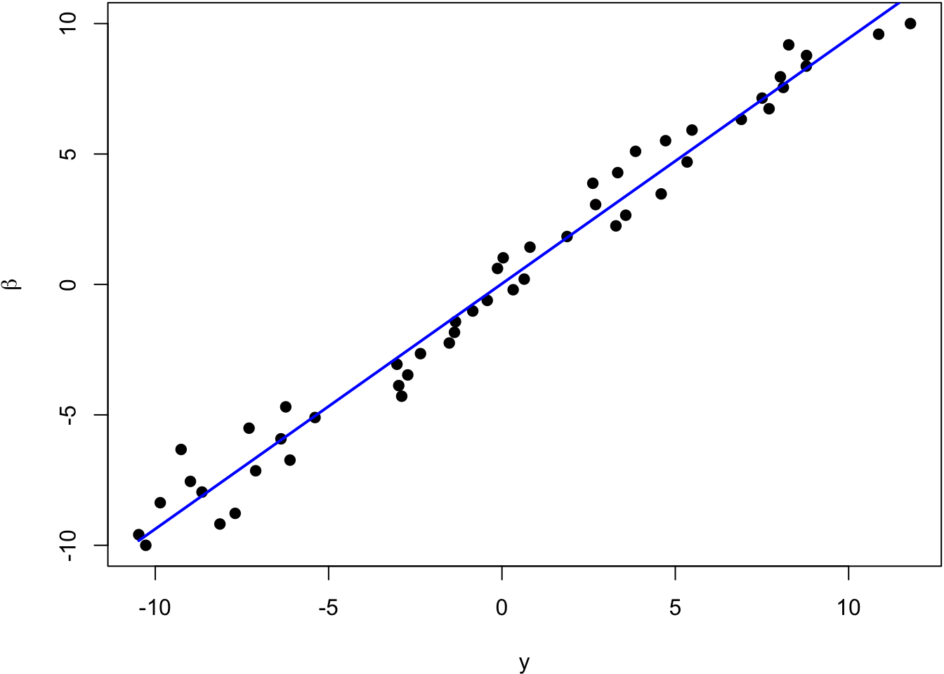
> beta <- seq(-10, 10, length.out=50)
> y <- beta + rnorm(length(beta))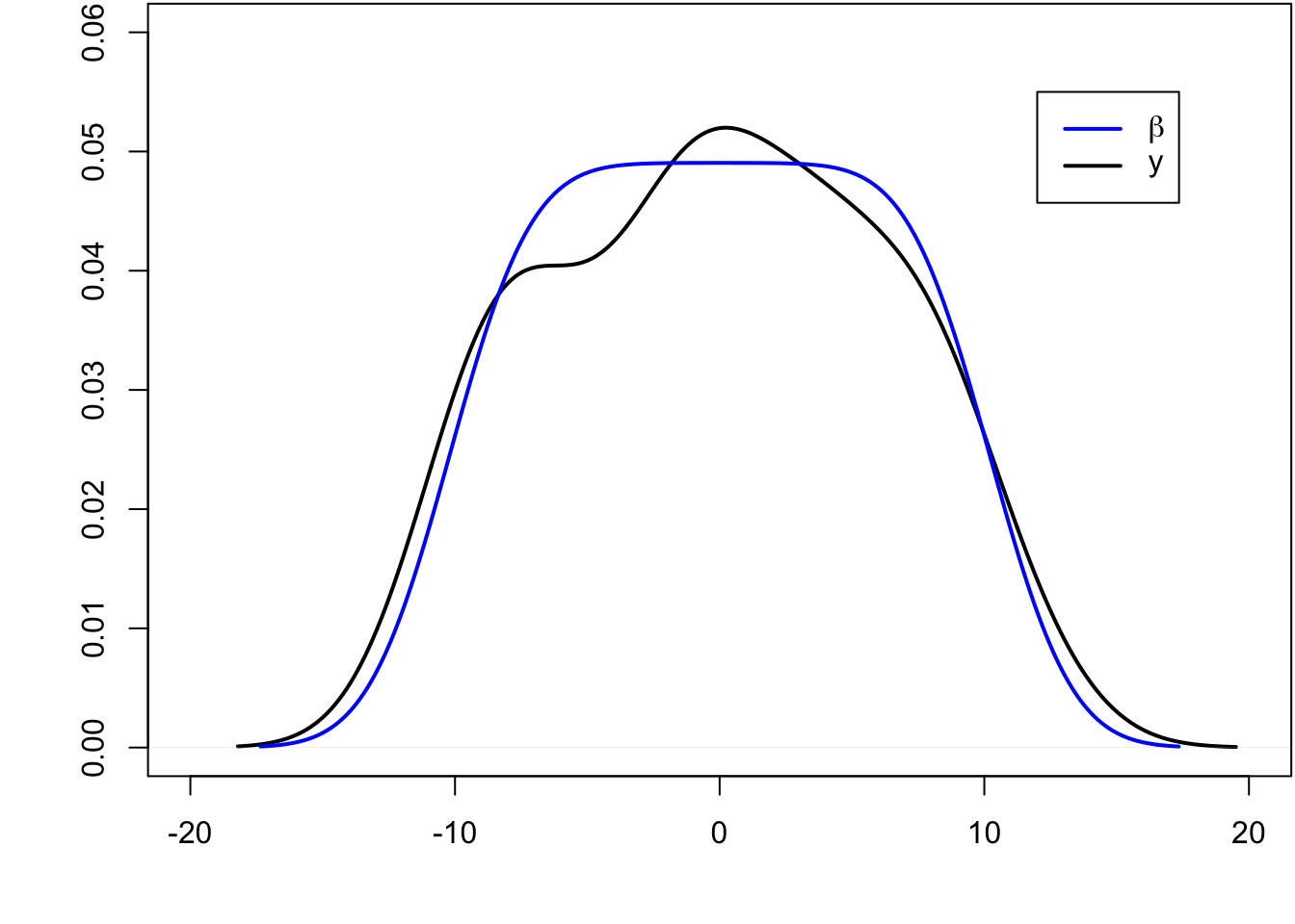

The blue line is the least squares regression line.

72.5 Inverse Regression Approach

While \(Y_i = \beta_i + E_i\) where \(E_i \sim \mbox{Normal}(0,1)\), it is also the case that \(\beta_i = Y_i - E_i\) where \(-E_i \sim \mbox{Normal}(0,1)\).

Even though we’re assuming the \(\beta_i\) are fixed, suppose we imagine for the moment that the \(\beta_i\) are random and take a least squares appraoch. We will try to estimate the linear model

\[ {\operatorname{E}}[\beta_i | Y_i] = a + b Y_i. \]

Why would we do this? The loss function is

\[ \sum_{i=1}^m (\beta_i - \hat{\beta}_i)^2 \]

so it makes sense to estimate \(\beta_i\) by setting \(\hat{\beta}_i\) to a regression line.

The least squares solution tells us to set

\[ \begin{aligned} \hat{\beta}_i & = \hat{a} + \hat{b} Y_i \\ & = (\bar{\beta} - \hat{b} \bar{Y}) + \hat{b} Y_i \\ & = \bar{\beta} + \hat{b} (Y_i - \bar{Y}) \end{aligned} \]

where

\[ \hat{b} = \frac{\sum_{i=1}^m (Y_i - \bar{Y})(\beta_i - \bar{\beta})}{\sum_{i=1}^m (Y_i - \bar{Y})^2}. \]

We can estimate \(\bar{\beta}\) with \(\bar{Y}\) since \({\operatorname{E}}[\bar{\beta}] = {\operatorname{E}}[\bar{Y}]\).

We also need to find an estimate of \(\sum_{i=1}^m (Y_i - \bar{Y})(\beta_i - \bar{\beta})\). Note that

\[ \beta_i - \bar{\beta} = Y_i - \bar{Y} - (E_i + \bar{E}) \]

so that

\[ \begin{aligned} \sum_{i=1}^m (Y_i - \bar{Y})(\beta_i - \bar{\beta}) = & \sum_{i=1}^m (Y_i - \bar{Y})(Y_i - \bar{Y}) \\ & + \sum_{i=1}^m (Y_i - \bar{Y})(E_i - \bar{E}) \end{aligned} \]

Since \(Y_i = \beta_i + E_i\) it follows that

\[ {\operatorname{E}}\left[\sum_{i=1}^m (Y_i - \bar{Y})(E_i - \bar{E})\right] = {\operatorname{E}}\left[\sum_{i=1}^m (E_i - \bar{E})(E_i - \bar{E})\right] = m-1. \]

Therefore,

\[ {\operatorname{E}}\left[\sum_{i=1}^m (Y_i - \bar{Y})(\beta_i - \bar{\beta})\right] = {\operatorname{E}}\left[\sum_{i=1}^m (Y_i - \bar{Y})^2 - (m-1)\right]. \]

This yields

\[ \hat{b} = \frac{\sum_{i=1}^m (Y_i - \bar{Y})^2 - (m-1)}{\sum_{i=1}^m (Y_i - \bar{Y})^2} = 1 - \frac{m-1}{\sum_{i=1}^m (Y_i - \bar{Y})^2} \]

and

\[ \hat{\beta}_i^{\text{IR}} = \bar{Y} + \left(1 - \frac{m-1}{\sum_{i=1}^m (Y_i - \bar{Y})^2}\right) (Y_i - \bar{Y}) \]

If instead we had started with the no intercept model

\[ {\operatorname{E}}[\beta_i | Y_i] = b Y_i. \]

we would have ended up with

\[ \hat{\beta}_i^{\text{IR}} = \left(1 - \frac{m-1}{\sum_{i=1}^m (Y_i - \bar{Y})^2}\right) Y_i \]

In either case, it can be shown that

\[ R\left({\boldsymbol{\beta}}, \hat{{\boldsymbol{\beta}}}^{\text{IR}}\right) < R\left({\boldsymbol{\beta}}, \hat{{\boldsymbol{\beta}}}^{\text{MLE}}\right). \]

The blue line is the least squares regression line of \(\beta_i\) on \(Y_i\), and the red line is \(\hat{\beta}_i^{\text{IR}}\).

72.6 Empirical Bayes Estimate

Suppose that \(Y_i | \beta_i \sim \mbox{Normal}(\beta_i, 1)\) where these rv’s are jointly independent. Also suppose that \(\beta_i {\; \stackrel{\text{iid}}{\sim}\;}\mbox{Normal}(a, b^2)\). Taking the empirical Bayes approach, we get:

\[ f(y_i ; a, b) = \int f(y_i | \beta_i) f(\beta_i; a, b) d\beta_i \sim \mbox{Normal}(a, 1+b^2). \]

\[ \implies \hat{a} = \overline{Y}, \ 1+\hat{b}^2 = \frac{\sum_{k=1}^m (Y_k - \overline{Y})^2}{n} \]

\[ \begin{aligned} {\operatorname{E}}[\beta_i | Y_i] & = \frac{1}{1+b^2}a + \frac{b^2}{1+b^2}Y_i \implies \\ & \\ \hat{\beta}_i^{\text{EB}} & = \hat{{\operatorname{E}}}[\beta_i | Y_i] = \frac{1}{1+\hat{b}^2}\hat{a} + \frac{\hat{b}^2}{1+\hat{b}^2}Y_i \\ & = \frac{m}{\sum_{k=1}^m (Y_k - \overline{Y})^2} \overline{Y} + \left(1-\frac{m}{\sum_{k=1}^m (Y_k - \overline{Y})^2}\right) Y_i \end{aligned} \]

As with \(\hat{{\boldsymbol{\beta}}}^{\text{JS}}\) and \(\hat{{\boldsymbol{\beta}}}^{\text{IR}}\), we have

\[ R\left({\boldsymbol{\beta}}, \hat{{\boldsymbol{\beta}}}^{\text{EB}}\right) < R\left({\boldsymbol{\beta}}, \hat{{\boldsymbol{\beta}}}^{\text{MLE}}\right). \]

72.7 EB for a Many Responses Model

Consider the many responses model where \({\boldsymbol{Y}}_{i} | {\boldsymbol{X}}\sim \mbox{MVN}_n({\boldsymbol{\beta}}_i {\boldsymbol{X}}, \sigma^2 {\boldsymbol{I}})\) where the vectors \({\boldsymbol{Y}}_{i} | {\boldsymbol{X}}\) are jointly independent (\(i=1, 2, \ldots, m\)). Here we’ve made the simplifying assumption that the variance \(\sigma^2\) is equal across all responses, but this would not be generally true.

The OLS (and MLE) solution is

\[ \hat{{\boldsymbol{B}}}= {\boldsymbol{Y}}{\boldsymbol{X}}^T ({\boldsymbol{X}}{\boldsymbol{X}}^T)^{-1}. \]

Suppose we extend this so that \({\boldsymbol{Y}}_{i} | {\boldsymbol{X}}, {\boldsymbol{\beta}}_i \sim \mbox{MVN}_n({\boldsymbol{\beta}}_i {\boldsymbol{X}}, \sigma^2 {\boldsymbol{I}})\) and \({\boldsymbol{\beta}}_i {\; \stackrel{\text{iid}}{\sim}\;}\mbox{MVN}_d({\boldsymbol{u}}, {\boldsymbol{V}})\).

Since \(\hat{{\boldsymbol{\beta}}}_i | {\boldsymbol{\beta}}_i \sim \mbox{MVN}_d({\boldsymbol{\beta}}_i, \sigma^2({\boldsymbol{X}}{\boldsymbol{X}}^T)^{-1})\), it follows that marginally

\[ \hat{{\boldsymbol{\beta}}}_i {\; \stackrel{\text{iid}}{\sim}\;}\mbox{MVN}_d({\boldsymbol{u}}, \sigma^2({\boldsymbol{X}}{\boldsymbol{X}}^T)^{-1} + {\boldsymbol{V}}). \]

Therefore,

\[ \hat{{\boldsymbol{u}}} = \frac{\sum_{i=1}^m \hat{{\boldsymbol{\beta}}}_i}{m} \]

\[ \hat{{\boldsymbol{V}}} = \hat{{\operatorname{Cov}}}\left(\hat{{\boldsymbol{\beta}}}\right) - \hat{\sigma}^2({\boldsymbol{X}}{\boldsymbol{X}}^T)^{-1} \]

where \(\hat{{\operatorname{Cov}}}\left(\hat{{\boldsymbol{\beta}}}\right)\) is the \(d \times d\) sample covariance (or MLE covariance) of the \(\hat{{\boldsymbol{\beta}}}_i\) estimates.

Also, \(\hat{\sigma}^2\) is obtained by averaging the estimate over all \(m\) regressions.

We then do inference based on the prior distribution \({\boldsymbol{\beta}}_i {\; \stackrel{\text{iid}}{\sim}\;}\mbox{MVN}_d(\hat{{\boldsymbol{u}}}, \hat{{\boldsymbol{V}}})\). The posterior distribution of \({\boldsymbol{\beta}}_i | {\boldsymbol{Y}}, {\boldsymbol{X}}\) is MVN with mean

\[ \left(\frac{1}{\hat{\sigma}^2}({\boldsymbol{X}}{\boldsymbol{X}}^T) + \hat{{\boldsymbol{V}}}^{-1}\right)^{-1} \left(\frac{1}{\hat{\sigma}^2}({\boldsymbol{X}}{\boldsymbol{X}}^T) \hat{{\boldsymbol{\beta}}}_i + \hat{{\boldsymbol{V}}}^{-1} \hat{{\boldsymbol{u}}} \right) \]

and covariance

\[ \left(\frac{1}{\hat{\sigma}^2}({\boldsymbol{X}}{\boldsymbol{X}}^T) + \hat{{\boldsymbol{V}}}^{-1}\right)^{-1}. \]