68 Generalized Additive Models
68.1 Ordinary Least Squares
Recall that OLS estimates the model
\[ \begin{aligned} Y_i & = \beta_1 X_{i1} + \beta_2 X_{i2} + \ldots + \beta_p X_{ip} + E_i \\ & = {\boldsymbol{X}}_i {\boldsymbol{\beta}}+ E_i \end{aligned} \]
where \({\operatorname{E}}[{\boldsymbol{E}}| {\boldsymbol{X}}] = {\boldsymbol{0}}\) and \({\operatorname{Cov}}({\boldsymbol{E}}| {\boldsymbol{X}}) = \sigma^2 {\boldsymbol{I}}\).
68.2 Additive Models
The additive model (which could also be called “ordinary nonparametric additive regression”) is of the form
\[ \begin{aligned} Y_i & = s_1(X_{i1}) + s_2(X_{i2}) + \ldots + s_p(X_{ip}) + E_i \\ & = \sum_{j=1}^p s_j(X_{ij}) + E_i \end{aligned} \]
where the \(s_j(\cdot)\) for \(j = 1, \ldots, p\) are a set of nonparametric (or flexible) functions. Again, we assume that \({\operatorname{E}}[{\boldsymbol{E}}| {\boldsymbol{X}}] = {\boldsymbol{0}}\) and \({\operatorname{Cov}}({\boldsymbol{E}}| {\boldsymbol{X}}) = \sigma^2 {\boldsymbol{I}}\).
68.3 Backfitting
The additive model can be fit through a technique called backfitting.
- Intialize \(s^{(0)}_j(x)\) for \(j = 1, \ldots, p\).
- For \(t=1, 2, \ldots\), fit \(s_j^{(t)}(x)\) on response variable \[y_i - \sum_{k \not= j} s_k^{(t-1)}(x_{ij}).\]
- Repeat until convergence.
Note that some extra steps have to be taken to deal with the intercept.
68.4 GAM Definition
\(Y | {\boldsymbol{X}}\) is distributed according to an exponential family distribution. The extension of additive models to this family of response variable is called generalized additive models (GAMs). The model is of the form
\[ g\left({\operatorname{E}}[Y_i | {\boldsymbol{X}}_i]\right) = \sum_{j=1}^p s_j(X_{ij}) \]
where \(g(\cdot)\) is the link function and the \(s_j(\cdot)\) are flexible and/or nonparametric functions.
68.5 Overview of Fitting GAMs
Fitting GAMs involves putting together the following three tools:
- We know how to fit a GLM via IRLS
- We know how to fit a smoother of a single explanatory variable via a least squares solution, as seen for the NCS
- We know how to combine additive smoothers by backfitting
68.6 GAMs in R
Three common ways to fit GAMs in R:
- Utilize
glm()on explanatory variables constructed fromns()orbs() - The
gamlibrary - The
mgcvlibrary
68.7 Example
> set.seed(508)
> x1 <- seq(1, 10, length.out=50)
> n <- length(x1)
> x2 <- rnorm(n)
> f <- 4*log(x1) + sin(x1) - 7 + 0.5*x2
> p <- exp(f)/(1+exp(f))
> summary(p)
    Min.  1st Qu.   Median     Mean  3rd Qu.     Max.
0.001842 0.074171 0.310674 0.436162 0.860387 0.944761
> y <- rbinom(n, size=1, prob=p)
> mean(y)
[1] 0.42
> df <- data.frame(x1=x1, x2=x2, y=y)
Here, we use the gam() function from the mgcv library. It automates choosing the smoothness of the splines.
> library(mgcv)
> mygam <- gam(y ~ s(x1) + s(x2), family = binomial(), data=df)
> library(broom)
> tidy(mygam)
# A tibble: 2 x 5
  term    edf ref.df statistic p.value
  <chr> <dbl>  <dbl>     <dbl>   <dbl>
1 s(x1)  1.87   2.37     12.7  0.00531
2 s(x2)  1.00   1.00      1.16 0.281
> summary(mygam)
Family: binomial
Link function: logit
Formula:
y ~ s(x1) + s(x2)
Parametric coefficients:
Estimate Std. Error z value Pr(>|z|)
(Intercept) -1.1380 0.6723 -1.693 0.0905 .
---
Signif. codes: 0 '***' 0.001 '**' 0.01 '*' 0.05 '.' 0.1 ' ' 1
Approximate significance of smooth terms:
edf Ref.df Chi.sq p-value
s(x1) 1.87 2.375 12.743 0.00531 **
s(x2) 1.00 1.000 1.163 0.28084
---
Signif. codes: 0 '***' 0.001 '**' 0.01 '*' 0.05 '.' 0.1 ' ' 1
R-sq.(adj) = 0.488 Deviance explained = 47%
UBRE = -0.12392 Scale est. = 1 n = 50True probabilities vs. estimated probabilities.
> plot(p, mygam$fitted.values, pch=19); abline(0,1)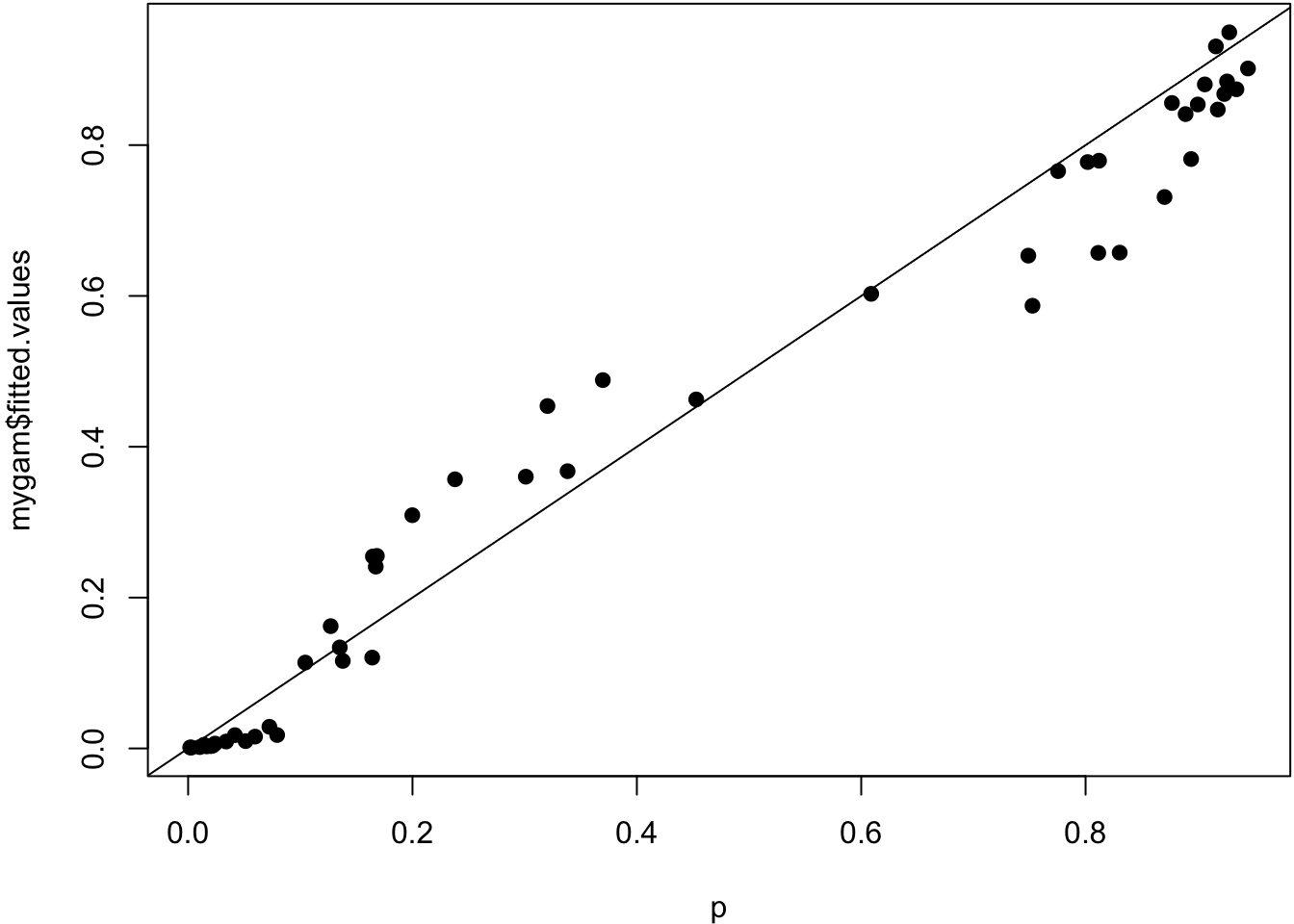
Smoother estimated for x1.
> plot(mygam, select=1)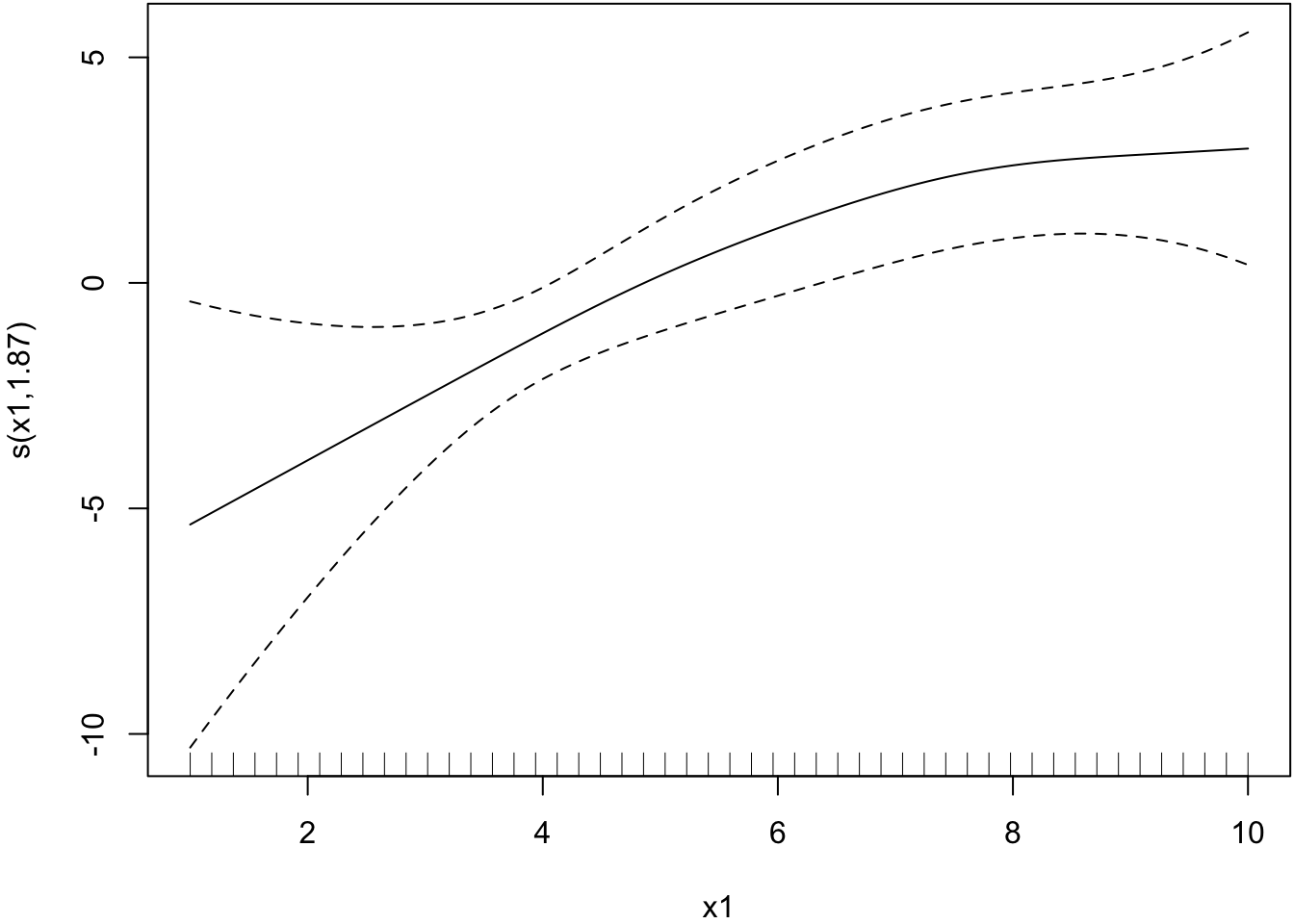
Smoother estimated for x2.
> plot(mygam, select=2)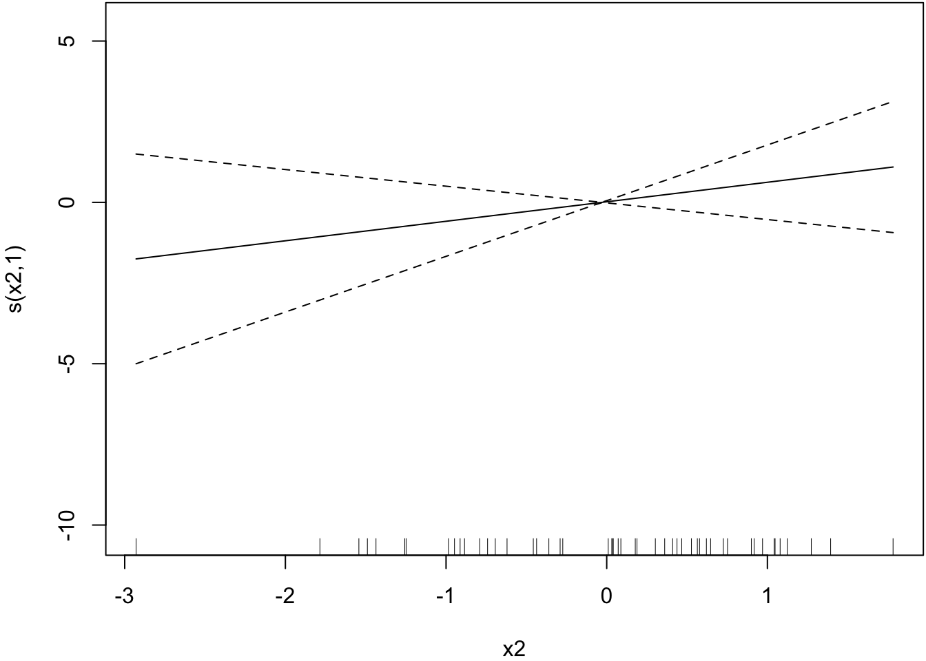
Here, we use the glm() function and include as an explanatory variable a NCS built from the ns() function from the splines library. We include a df argument in the ns() call.
> library(splines)
> myglm <- glm(y ~ ns(x1, df=2) + x2, family = binomial(), data=df)
> tidy(myglm)
# A tibble: 4 x 5
term estimate std.error statistic p.value
<chr> <dbl> <dbl> <dbl> <dbl>
1 (Intercept) -10.9 5.31 -2.06 0.0396
2 ns(x1, df = 2)1 21.4 10.1 2.11 0.0348
3 ns(x1, df = 2)2 6.33 2.11 3.00 0.00272
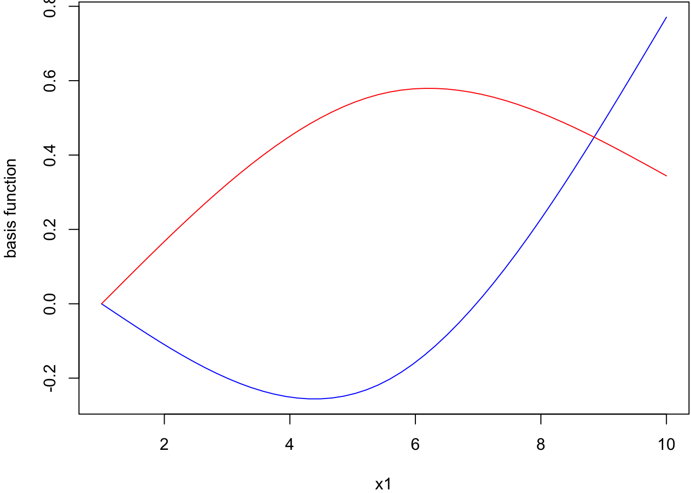
4 x2 0.734 0.609 1.21 0.228 The spline basis evaluated at x1 values.
> ns(x1, df=2)
               1           2
 [1,] 0.00000000  0.00000000
 [2,] 0.03114456 -0.02075171
 [3,] 0.06220870 -0.04138180
 [4,] 0.09311200 -0.06176867
 [5,] 0.12377405 -0.08179071
 [6,] 0.15411442 -0.10132630
 [7,] 0.18405270 -0.12025384
 [8,] 0.21350847 -0.13845171
 [9,] 0.24240131 -0.15579831
[10,] 0.27065081 -0.17217201
[11,] 0.29817654 -0.18745121
[12,] 0.32489808 -0.20151430
[13,] 0.35073503 -0.21423967
[14,] 0.37560695 -0.22550571
[15,] 0.39943343 -0.23519080
[16,] 0.42213406 -0.24317334
[17,] 0.44362840 -0.24933170
[18,] 0.46383606 -0.25354429
[19,] 0.48267660 -0.25568949
[20,] 0.50006961 -0.25564569
[21,] 0.51593467 -0.25329128
[22,] 0.53019136 -0.24850464
[23,] 0.54275927 -0.24116417
[24,] 0.55355797 -0.23114825
[25,] 0.56250705 -0.21833528
[26,] 0.56952943 -0.20260871
[27,] 0.57462513 -0.18396854
[28,] 0.57787120 -0.16253131
[29,] 0.57934806 -0.13841863
[30,] 0.57913614 -0.11175212
[31,] 0.57731586 -0.08265339
[32,] 0.57396762 -0.05124405
[33,] 0.56917185 -0.01764570
[34,] 0.56300897  0.01802003
[35,] 0.55555939  0.05563154
[36,] 0.54690354  0.09506722
[37,] 0.53712183  0.13620546
[38,] 0.52629468  0.17892464
[39,] 0.51450251  0.22310315
[40,] 0.50182573  0.26861939
[41,] 0.48834478  0.31535174
[42,] 0.47414005  0.36317859
[43,] 0.45929198  0.41197833
[44,] 0.44388099  0.46162934
[45,] 0.42798748  0.51201003
[46,] 0.41169188  0.56299877
[47,] 0.39507460  0.61447395
[48,] 0.37821607  0.66631397
[49,] 0.36119670  0.71839720
[50,] 0.34409692  0.77060206
attr(,"degree")
[1] 3
attr(,"knots")
50%
5.5
attr(,"Boundary.knots")
[1]  1 10
attr(,"intercept")
[1] FALSE
attr(,"class")
[1] "ns"     "basis"  "matrix"
Plot of basis function values vs x1.
> summary(myglm)

Call:
glm(formula = y ~ ns(x1, df = 2) + x2, family = binomial(), data = df)

Deviance Residuals:
    Min       1Q   Median       3Q      Max
-2.0214  -0.3730  -0.0162   0.5762   1.7616

Coefficients:
                Estimate Std. Error z value Pr(>|z|)
(Intercept)     -10.9229     5.3079  -2.058  0.03960 *
ns(x1, df = 2)1  21.3848    10.1318   2.111  0.03480 *
ns(x1, df = 2)2   6.3266     2.1103   2.998  0.00272 **
x2                0.7342     0.6089   1.206  0.22795
---
Signif. codes:  0 '***' 0.001 '**' 0.01 '*' 0.05 '.' 0.1 ' ' 1

(Dispersion parameter for binomial family taken to be 1)

    Null deviance: 68.029  on 49  degrees of freedom
Residual deviance: 35.682  on 46  degrees of freedom
AIC: 43.682

Number of Fisher Scoring iterations: 7
> anova(myglm, test="LRT")
Analysis of Deviance Table
Model: binomial, link: logit
Response: y
Terms added sequentially (first to last)
Df Deviance Resid. Df Resid. Dev Pr(>Chi)
NULL 49 68.029
ns(x1, df = 2) 2 30.755 47 37.274 2.097e-07 ***
x2 1 1.592 46 35.682 0.207
---
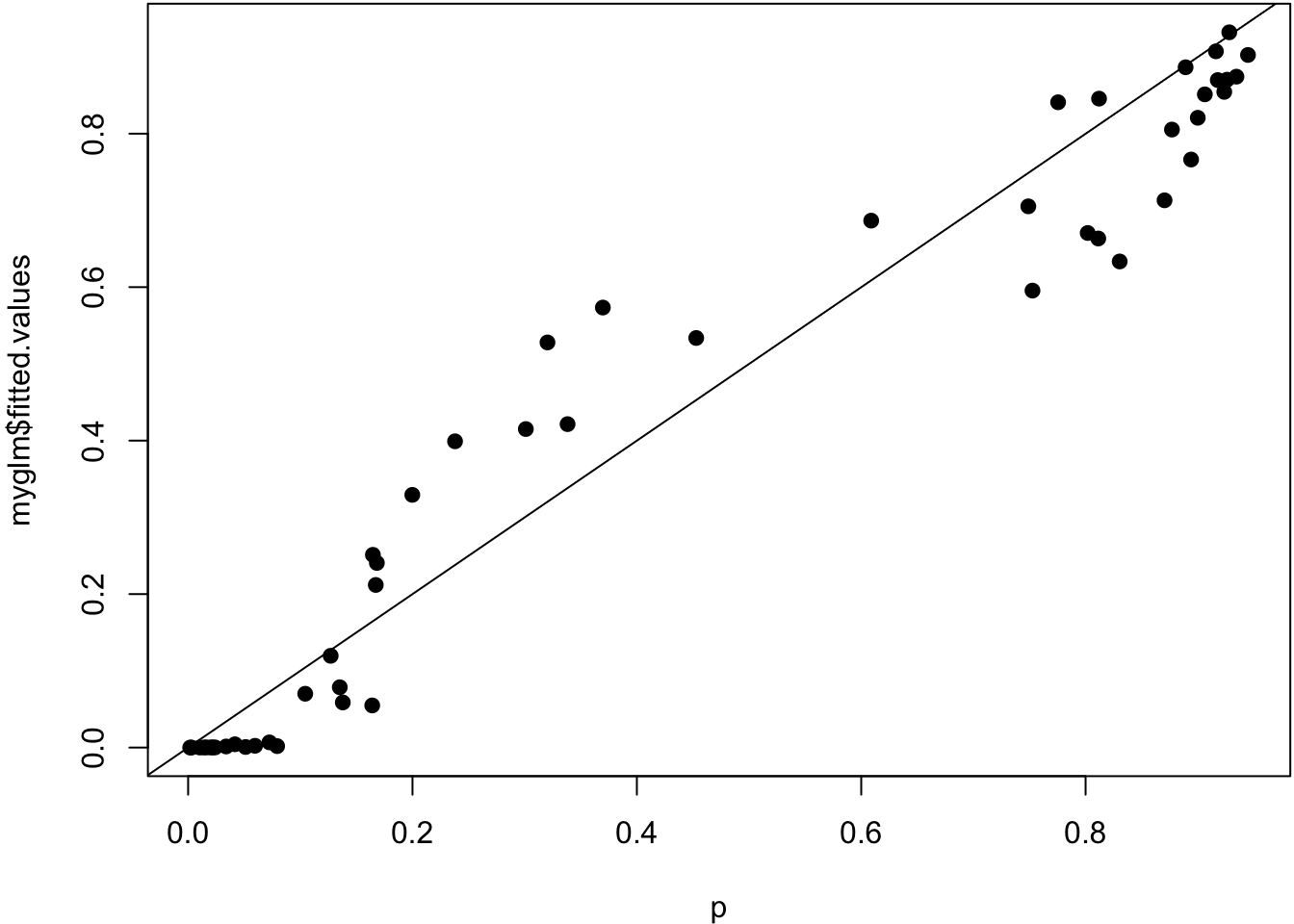
Signif. codes: 0 '***' 0.001 '**' 0.01 '*' 0.05 '.' 0.1 ' ' 1True probabilities vs. estimated probabilities.
> plot(p, myglm$fitted.values, pch=19); abline(0,1)